Introduction
Location Map
Base Map
Database Schema
Conventions
GIS Analyses
Flowchart
GIS Concepts
Results
Conclusion
References

GIS Analyses

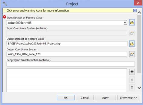
Cober2005_projected
Land cover file was re-projected to WGS 1984 UTM Zone 17 N

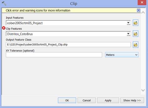
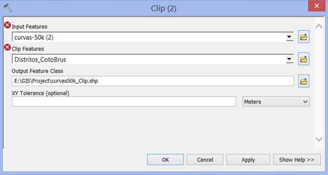
Once re-projected, the land cover file was clipped into the Districts shapefile of Coto Brus County

The Topographic curves obtained from the Organization for Tropical Studies (OTS) was also clipped into Districts shapefile.

DEM
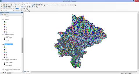
The clipped Topographic file was first converted into a Raster by using the Conversion Tool of Polyline to Raster.

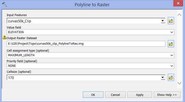
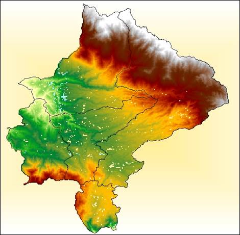
However, such tool was not successful as shown in the following map where white spaces were not filled into the DEM.

Our second approach was by using an interpolation tool from the spatial analyst toolbox, called Topo to Raster.

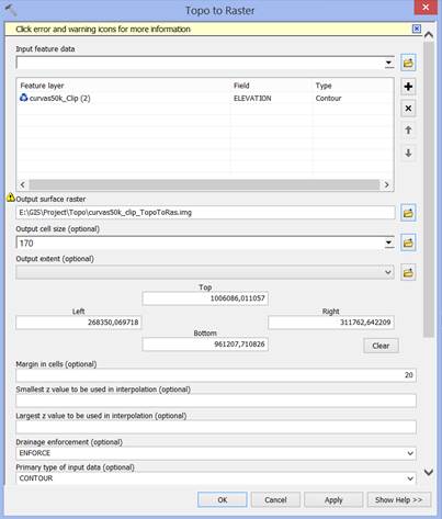
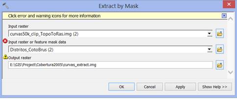
The raster created from the Topographic data was extracted by mask into the Districts of Coto Brus County. This file was used as the final DEM for the rest of the processes.

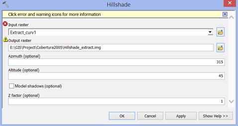
The DEM was then hillshaded

NDVI

All the Landsat data was downloaded from http://earthexplorer.usgs.gov, to calculate the Normalized Difference Vegetation Index (NDVI). We selected two images, one from February 16th, 1998, and another one from April 1st, 2014, to try to detect difference in the vegetation for Coto Brus county. Landsat 5 TM at 30 m resolution was used to compose 1998 map, using bands 1 to 7, excluding band 6 because it’s a thermal infrared at 120 m resolution. Landsat 8 OLI at 30 m resolution was used to compose 2014 map, using bands 2 to 7. (http://landsat.usgs.gov/band_designations_landsat_satellites.php).
Bands 3 and 4 were used to create NDVI. We used Landsat5 to compose 1998 map because Landsat7 data has striping issues in our area of interest. We used Landsat 8 to compose 2014 map because Landsat 5 only have data till 2011.
Data Acquisition
1. At the home page of http://earthexplorer.usgs.gov zoom in till you find Costa Rica, then look for Coto Brus. Click Go.
2. Choose the Landsat 4-5 TM Collection at a Resolution of 30m.
3. Select scenes that appear cloud-free enough around Coto Brus, and Add to Scene List. Create a free cart to download the data.
4. Repeat step 2 and 3 for Landsat 8 OLI at Resolution of 30 m. The folder selected were: LT50140541998047CPE03.tar and LC80140542014091LGN00.tar. For the last folder, for example, 2014 is the year and 091 is the Julian date.
5. Data downloads in .tar format.
6. Use a program such as 7-Zip File Manager to unzip each folder.
Data Preparation
1. Open ArcCatalog, and connect to folders where the unzip Landsat 5 and Landsat 8 bands are saved.
2. Open blank map in ArcMap.
3. Add Data. Add the Landsat 5 and 8 bands to your map document.
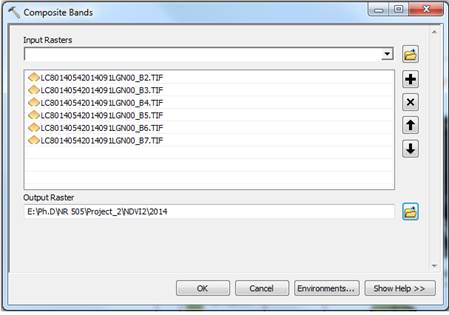
4. ArcToolbox --> Data Management --> Raster --> Raster Processing--> Composite Bands. Select the bands from Landsat 8, and save the raster with a meaningful name, in this case, 2014. Do the same for Landsat 5 bands, and save the raster as 1998.

5. Landsat 8 band combinations differ from Landsat 5 satellite data.

http://landsat.usgs.gov/L8_band_combos.php
We changed the color images to false color or color infra-red. So, for Landsat 5 we set:
Red = Layer 4
Green = Layer 3
Blue = Layer 2

And for Landsat 8, we set:
Red = Layer 5
Green = Layer43
Blue = Layer 3

Darker green indicates healthy vegetation and red-bluish colors are either less vegetation, urban areas or water.

Data Analysis
1. Click on Windows --> Image Analysis.
-In the Image Analysis window, click on the 1998 image.
-Click on the Image Analysis option button. Set Red Band in 3, and Infrared Band in 4, which are the default options. Click on the check boxes for Use Wavelength and Scientific Ouptut.
- -Click on the NDVI icon . Change the color ramp to “Purple to Green Diverging, Dark” (this is similar to the standard NDVI color scheme).
-Repeat this procedure for 2014 image.
-As result, we created two new images, NDVI 1998 and NDVI 2014
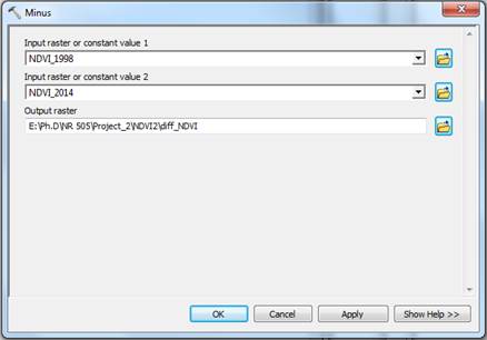
2. To analyze the change in land cover between NDVI 1998 and NDVI 2014, we used the function Minus, from the Spatial Analyst Math. It simply subtracts one image (1998, in this case) from another (2014).

3. We use the function Extract by Mask for the new map diff_NDVI using Coto Brus.shp, so the map only showed the change in vegetation for Coto Brus county.
4. We converted diff_NDVI into two classes – one representing negative values, which generally indicate less vegetation and positive values that indicate more vegetation. For that, we used a classification technique.
-Go to Customize --> Toolbars, and select Image Classification.

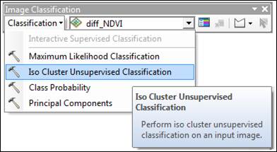
-Click on the Classification dropdown menu, and select Iso Cluster Unsuperivsed Classification. Then, select the diff_NDVI, set the number of classes to 2. Give your output a meaningful name, in this case, “isocluster”. Accept the defaults for minimum class and sample interval. Finally, give a meaningful name for your signature file.
In this step we created a layer that identifies 1 as less vegetation (our negative numbers) and 2 as more vegetation (our positive numbers).
We clipped isocluster to the Coto Brus shapefile, so the following calculations were only for the area of interest. The clipped file name was “clip_iso2”.
Then, we measured the difference in change between less vegetation and more vegetation by converting out raster output of two classes to polygon:
-Conversion --> From Raster --> Raster to Polygon. We obtained a shapefile that was named “clipiso2_poly.shp”.
-We opened the attribute table of clipiso2_poly.shp, and added a field called Hectares. We made it a Float. Then, right clicked on Hectares and Calculate Geometry (selecting hectares).
-Then, we
summarized the Gridcode field by the Hectares field. Choosed sum.
-Finaly, we obtained a table that quantified the change based on the difference between NDVI_1998 and NDVI_2014.

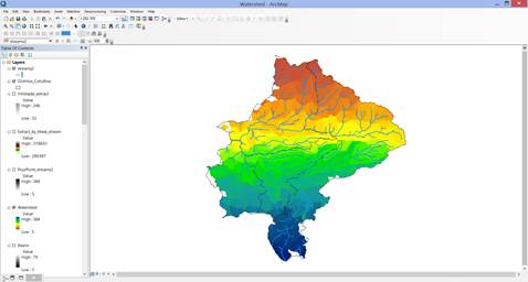
Watershed
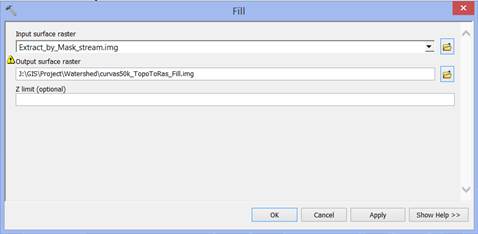
The DEM was clipped into the AOI and the Flow Direction tool was run, creating an output with 14 directions which means that some sinks could be present in the DEM. The sinks were filled in by using the Fill tool from the Spatial Analyst toolbox. This tool removes the small imperfections in the data.

A second Flow Direction was run, showing the 8 directions that are expected from the tool.

The flow direction was used to create a flow accumulation.

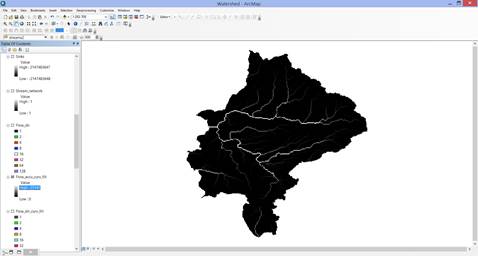
The same flow direction was used to create features out of the streams drawn by the program as well as the watershed.

Slope Pastureland

Selection by attributes from cober2005crtm05_Project_clip.shp → Cobertura=No Forestal (Pastureland).

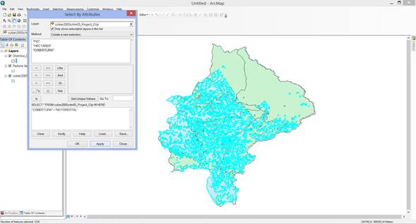
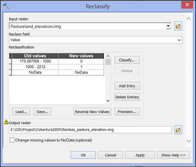
Creating a new shape file out of the pastureland selection called pastureland. Pastureland in Coto Brus comprises 34348 hectares that are scattered in an area of about 273651 hectares. Pastureland shape file and curvas_extract raster were extracted by mask into a new raster called pastureland elevation

Pastureland_elevation raster showing the range of elevation for the pastureland cover in Coto Brus County.

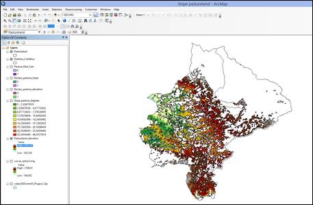
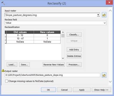
The pastureland_elevation raster was used to estimate the slope in degrees

Slope_pasture_degrees raster showed slopes in a range from 0 to 46 degrees.

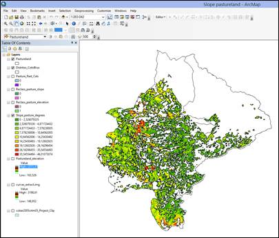
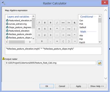
Both pastureland_elevation and slope_pasture_degrees were reclassified into two categories to show areas with elevation higher than a 1000 m, and slopes higher than 10 degrees, respectively. The criteria used to reclassify both rasters were based on taking about half of the elevation for the pastureland in the AOI. The slope >10 degrees might seem a little conservative, however, due to the high level of precipitation in the AOI, landslides, erosion and, runoff may occur even with a lower degree of slope. Mwendera et al. (1997) analyzed different grazing pressures in pastures with two slopes (0-4% and 4-8%) and found that the biomass is affected similarly in both sites (slopes) but, the areas with higher slopes can be severely affected with a light grazing pressure.

The raster calculator tool was used to estimate the areas that meet the requirements of high elevation and high slope established for the reclassified slope and elevation raster files.