Introduction
Location Map
Base Map
Database Schema
Conventions
GIS Analyses
Flowchart
GIS Concepts
Results
Conclusion
References

Results

Results of the Control Group

General results, by group

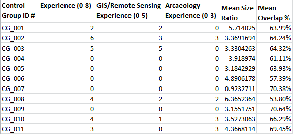
Surprisingly, the human control group performed better than the computer algorithm in overlapping their complejo boundaries with the boundaries on the original map (64.14%, standard deviation 12.79%). However, this result becomes unsurprising when size ratio is taken into account: the participants tended to draw their complejo boundaries approximately four times larger than the original complejo boundaries (3.886, standard deviation 4.89). Therefore, this analysis suggests that humans are not reliable when it comes to drawing boundaries. The implications of this are noteworthy, since, outside of the ground-truthed area, boundaries were drawn by hand in GIS.

Another interesting result is that one of the participants with no GIS, remote sensing, or archaeology experience had complejo boundaries that most closely match the original map (70.38% mean overlap percentage, .923 mean size ratio).

General results, by complejo

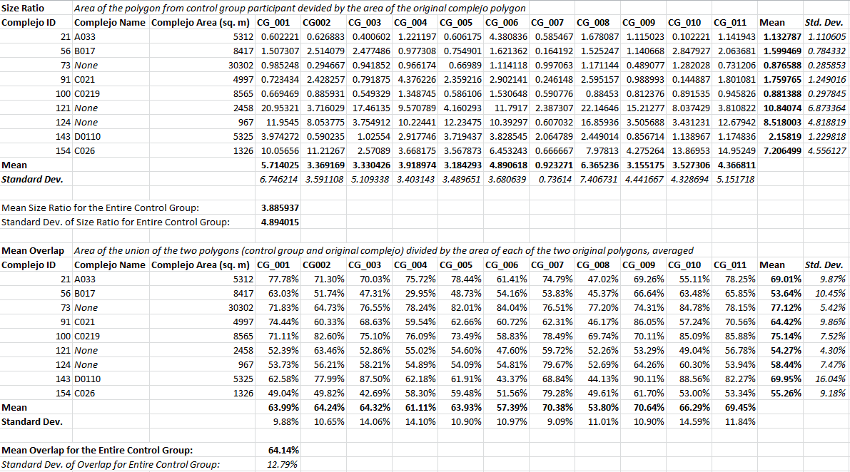
It seems that the participant complejo boundaries that best matched the original map were 73 and 100.

Complejo 73

Participant boundaries of complejo 73 had a .876 size ratio and 77.12% mean overlap. This means that most participants drew their complejo smaller than the original, but mostly overlapping. Some possible explanations for this are the very clearly defined road to the left of the complejo and the cliff to the right, a major topographic change. These major boundary definers made this particular complejo boundary the easiest to draw out of the nine.

Complejo 100

Participant boundaries for complejo 100 were even closer to the original map, with a .881 size ratio, but a slightly lower mean overlap percentage, at 75.14%. Possible reasons for the ease in creating this boundary could include the road, the plaza, and the general �grouped� nature of the structures.

In contrast, participant complejo boundaries for 121 and 124 were much further off from the original map.

Complejo 121

Participant boundaries for complejo 121 had an astonishing 10.841 size ratio and a 54.27% mean overlap. Participants drew this complejo, on average, ten times larger than the original, with some participants drawing it up to 20 times larger. A significant reason why complejo 121 may have been difficult to determine a boundary for is that higher elevation terrain is harder to differentiate features on. In this case, lava flow is younger in this region, which makes the terrain more jagged.

Complejo 124

Participant boundaries for complejo 124 had an 8.518 size ratio and a 58.44% mean overlap, which is only slightly better than the boundary drawing for complejo 121. Some possible explanations for the difficulty in creating this boundary are the plaza adjacent to the site and the level of topographic change in the area. Some participants included the plaza from the adjacent complejo, which easily doubles the size of complejo 124. Additionally, it is possible that participants extended their boundaries closer to the topographic changes, as this was described as a boundary-defining feature. However, doing this could quadruple the size of the complejo.

Results of the Multiresolution Segmentation

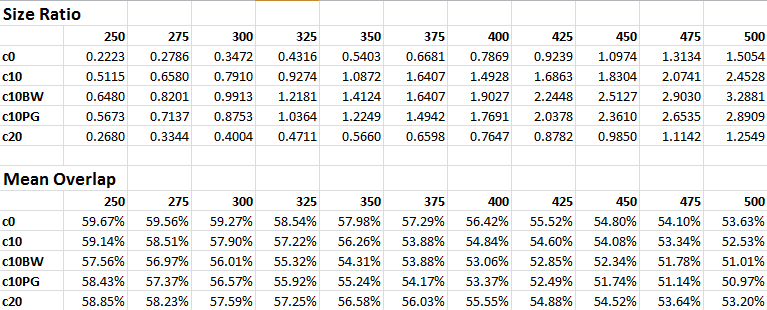
The results of the multiresolution segmentation are so far inconclusive. Of the various rasters used in the study, the most effective was the c10 raster, in which the DEM was symbolized using ESRI's Elevation #1 colors, with the color parameter set to 0.1 in the MRS algorithm. When compared to the entire complejo map, the output that fit best had the scale parameter at 325. This yielded results a size ratio of 0.92 and a mean overlap of 57.90%.

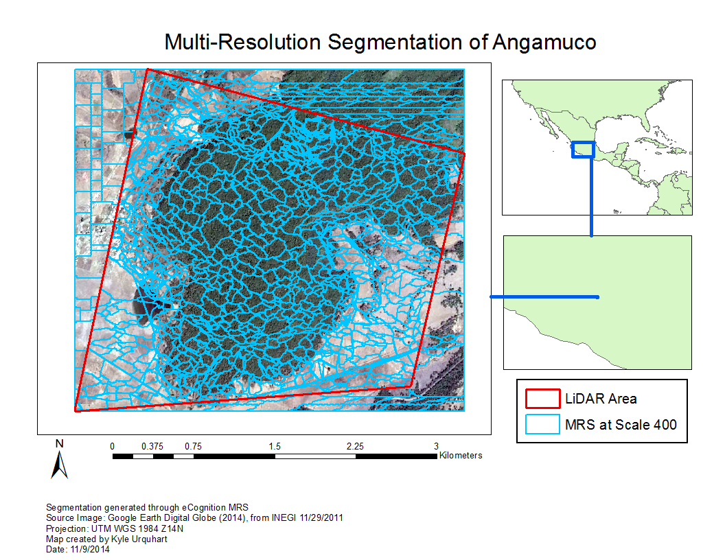
However, the results from the control group led us to question the utility of the original complejo map, as many of the complejos in that map were drawn using that method. So instead we created a second shape file containing only those complejos which have ground truthed survey data. When we compared the algorithm outputs to only these complejos, the best fit was at a scale parameter of 400. This yielded a mean size ratio of 0.98, with a standard deviation of 0.11, which was far more precise than any participant in the human control group. However, the mean overlap was only 59.93%, which is 20 percentage points short of the industry threshold of 80% for unsupervised classification. There are a number of ways that this may be improved, which will be discussed in the conclusion section. Nevertheless, within the scope of the study this output was the best fit. The segments from this output are shown below, overlaid on an image of the site taken from GoogleEarth.

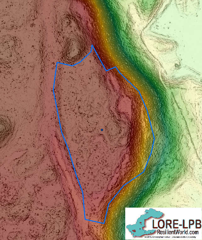
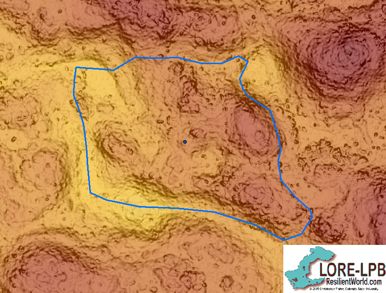
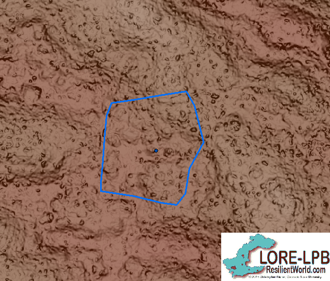
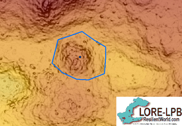
To place these results in a more qualitative context, the algorithm appears to do a great job highlighting boundaries when the boundaries are defined by major topographic changes, but it does not appear to be effective at detecting roads or plazas as boundaries. (See figure below).

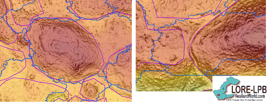
The image above shows two examples of how the algorithm recognizes boundaries. In the image on the left, the original complejo (in purple) was defined as located on a hill. Several small structures are visible on top of this hill, and the boundary of the complejo can be rather easily defined as the edge of the hill. The algorithm placed the boundary (blue) in almost the exact same place as the human observer, although it included a chunk to the northeast that was not included in the original. In the image on the right, a road forms the boundary of a complejo, which the algorithm did not recognize. If, at some point in the future, we find a way to easily detect roads and/or plazas in the LiDAR data, then the base raster could be modified to include that information and the algorithm would segment around them. Within the scope of this experiment, however, the algorithm was only provided topographic information and the segmentation reflects this.