Introduction
Location Map
Base Map
Database Schema
Conventions
GIS Analyses
Flowchart
GIS Concepts
Results
Conclusion
References

GIS Analyses

GIS Analyses

Small Datasets

For small datasets it may only be appropriate to use either TIN or Nearest Neighbor approaches. Here we show comparisons between these two interpolation techniques both visually and statistically, along with instructions on how to create these surfaces.

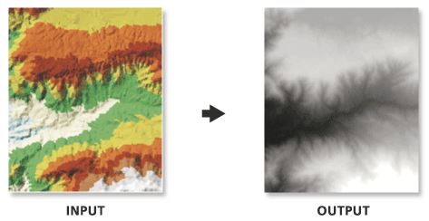
Point data, in this case elevation data, was used as the input feature for the Create TIN 3D Analyst tool. An input projected coordinate system is required for the Delaunay traingulation method to function properly. In this analysis NAD83 US State Plane Alaska zone 4 was used.

In order to compare this surface to other surface interpolation techniques, you must convert the TIN to a Raster, using the TIN to Raster 3D Analyst tool. This conversion, however, leads to a slight loss of data due to the irregular output of a TIN and the regular (grid) output of a raster.

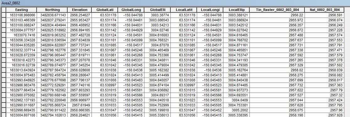
Once the data is in raster format, you can begin both visual and statistical comparisons. Statistical comparison of this surface technique begins by extracting the elevation/value the interpolation surface assigns a point and comparing that to the input data points elevation/value. The Extract (Multi)Values to Points tool extracts elevation data from the interpolated surface and joins this data to the Attribute Table of the input point data. This can then be exported to Excel and a root mean square analysis can be performed.

To understand this tool's ability to interpolate a surface based off of a point data set, a simplified version of the input point data was created. This was done by exporting every other point into a separate feature class and then repeated a second time. The output surfaces of this simplification are shown below (July 9th is on the left and August 2nd is on the right).

Again point data is used as the input feature for the Natural Neighbor Spatial Analyst or 3D Analyst tool. This tool creates a raster output in the same coordinate system as the input features, i.e. NAD83 US State Plane Alaska zone 4

Here the Extract (Multi)Values to Points tool was used again to obtain Natural Neighbor surface values to compare to the input point data.

A simplified version of the input point data was created. The output surfaces of this simplification are shown below (July 9th is on the left and August 2nd is on the right).

TIN and Natural Neighbor Comparison

To understand the capabilites and shortcomings of these two different surface tools, three different methods were used. One was mentioned above --the Extract Values to Points tool -- the second is the Surface Difference tool, and the third is Raster Calculator.

The Extract Values to Points tool as mentioned on theGIS Concepts page, joins the elevation values of the interpolated surface to the corresponding input point data. These values express the offset elevation that the interpolated surface has assigned to the input point. This can be visualized as a canvas being stretched across a table. If the table has nothing on it, the difference between the input data points and the interpolated surface will be minimal. However as you add items and complexities to the table's surface, the difference between the input data and the interpolated surface will increase. Thus this tool was used to help understand the interpolated surface's ability to effectively represent the point data.

The outputs from this tool for the original and simplified Nearest Neighbor and TIN surfaces were exported to a table in Excel.The difference between the input point elevation value and the output interpolated surface value for that point was squared and summed. These results are shown in Table 1 on theResults page.

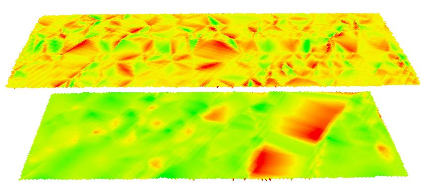
The second comparison between small dataset interpolation techniques was accomplished through the Surface Differencing tool. This tool provided a visual representation of the difference between TIN surfaces created for data collected during the two different time periods: July 9th and August 2nd. The images displayed below show the change in elevation from July 9th to August 2nd on the top, and August 2nd to July 9th on the bottom. On the left are the original TIN surfaces.

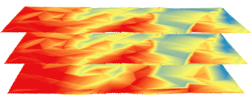
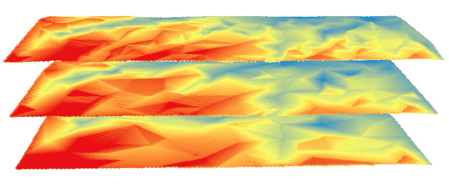
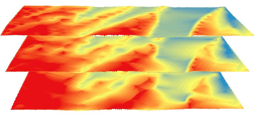
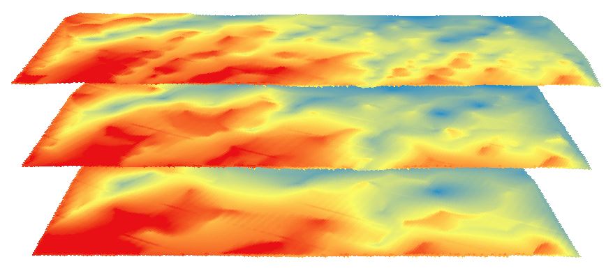
The third comparison method between these surfaces was completed using Raster Calculator. The increasingly simplified raster surfaces produced through the Natural Neighbor tool. The surfaces created using the Natural Neighbor technique were subtracted from one another to produce an output Raster. The produced surfaces are shown below. Areas shown in red are areas of elevation loss and areas shown in yellow are elevation gains. On the top is the difference between the original raster surface and the most simplified surface (_simple2); in the middle is the difference between the mid-level simplified surface (_simplified) and the most simplified surface; and on the bottom is the difference between original surface and the mid-level simplified surface.

To interpolate a surface using Kriging and IDW, the Geostatistical Analyst extension was used because of its ability to assess surfaces before moving on to further analyses. Because of the large amount of data in our "large" dataset, we were able to use the Subset feature to evaluate our results. With this method, one subset of the data was used to create the surface, then the surface was compared to the known values of the second subset.

The Geostatistical Wizard was used to produce both interpolated surfaces.

IDW Wizard:

After selecting "Inverse Distance Weighting" step 2 in the wizard allows for changes to be made to the power, neighbor numbers, etc.

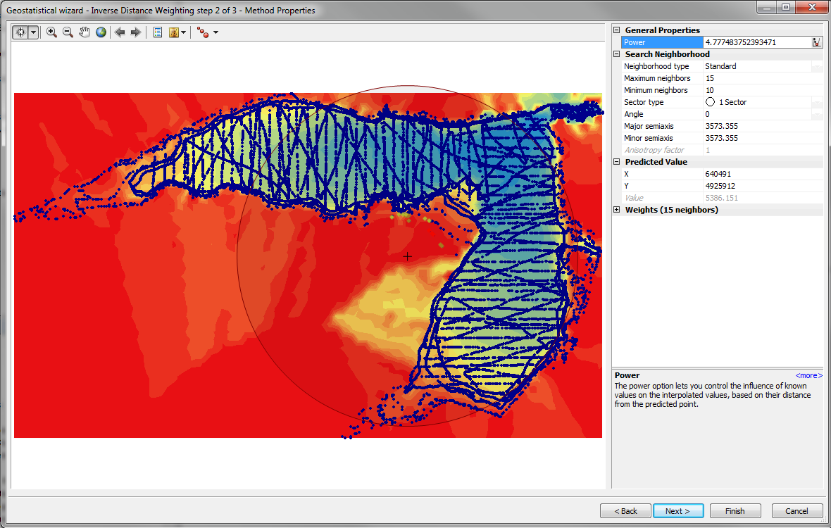
There is also a button to optimize parameters (power in the case of the above window)

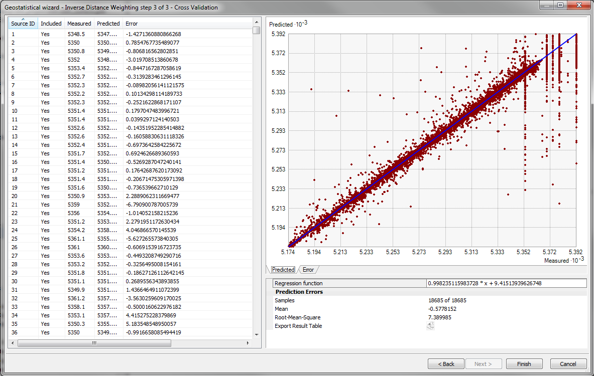
Step 3 in the wizard for IDw displays plots for cross validation and error:

Completion of the process in the wizard results in a sumary report:

Kriging Wizard:

The kriging wizard is much like the IDW wizard, but has a couple additional steps.

Step 1 and 2 involve selecting the method to use and the data that will be interpolated.

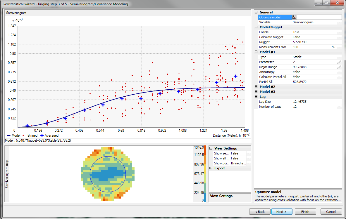
Step 3 allows for optimizing the model and seeing the model fit:

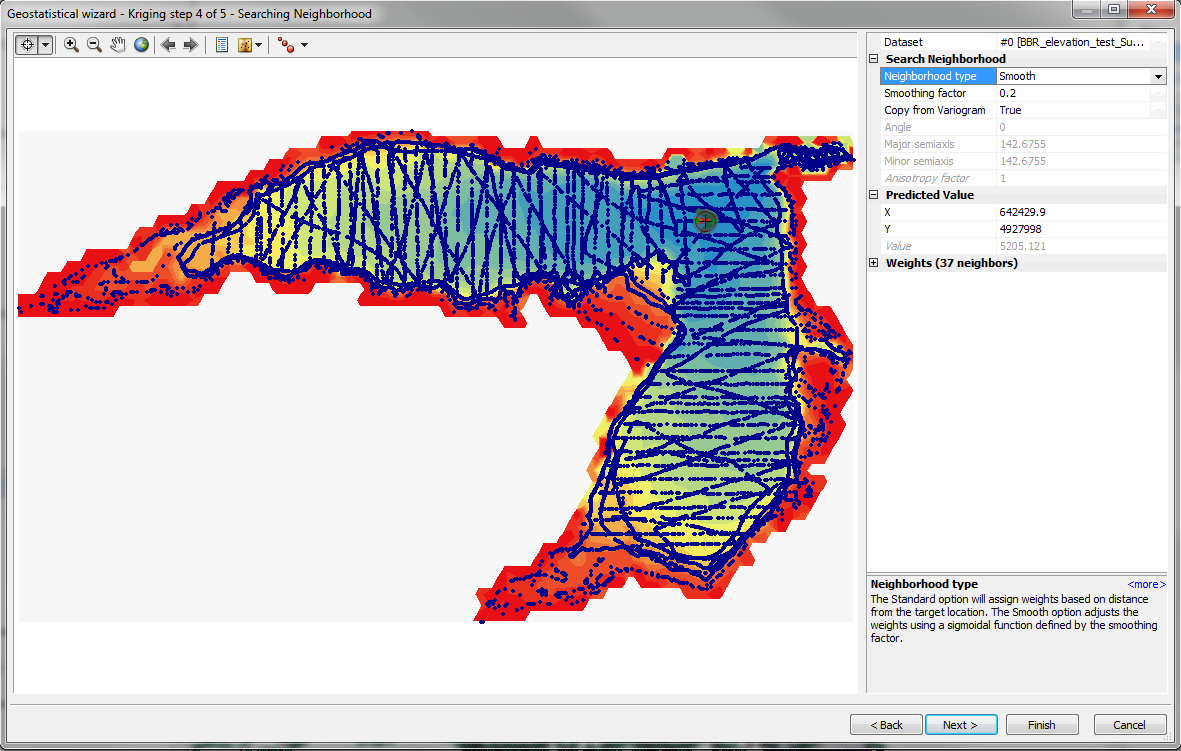
Step 4 allows adjustment to the search neighborhood and the smoothing factor:

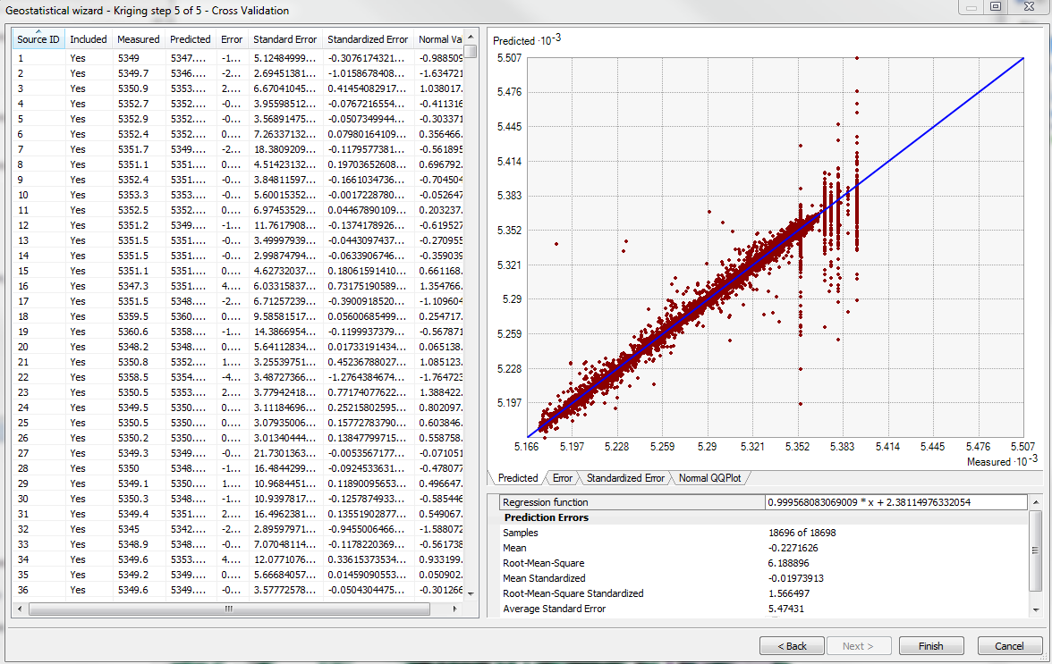
Again, the final step allows the us to view predicted values, error, standard error, and QQplots:

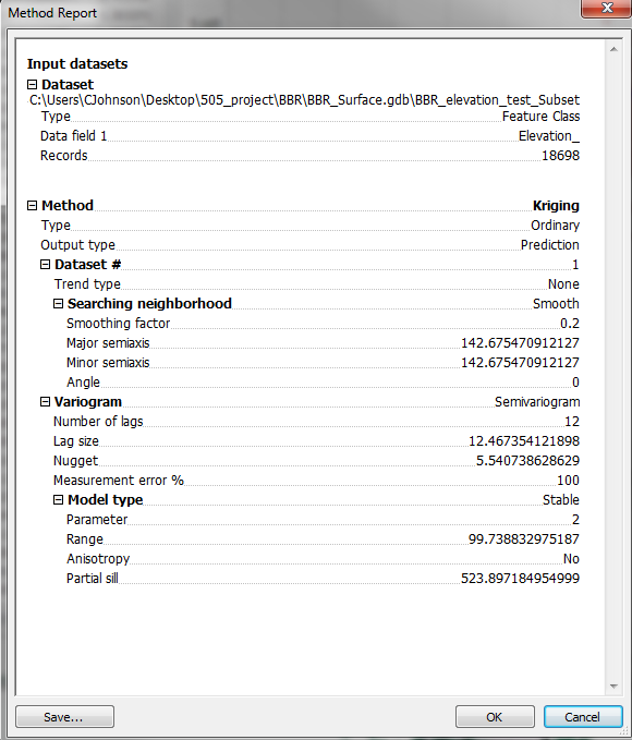
We also get a summary report for Kriging:

Comparison and Validation:

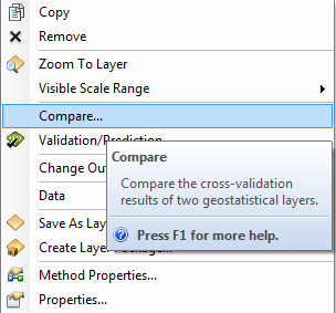
From the Geostatistical Analyst Extension, there are tools for Comparison and Validation/Prediction between at least two methods. These tools can be found by right clicking on the surface name in the table of contents:

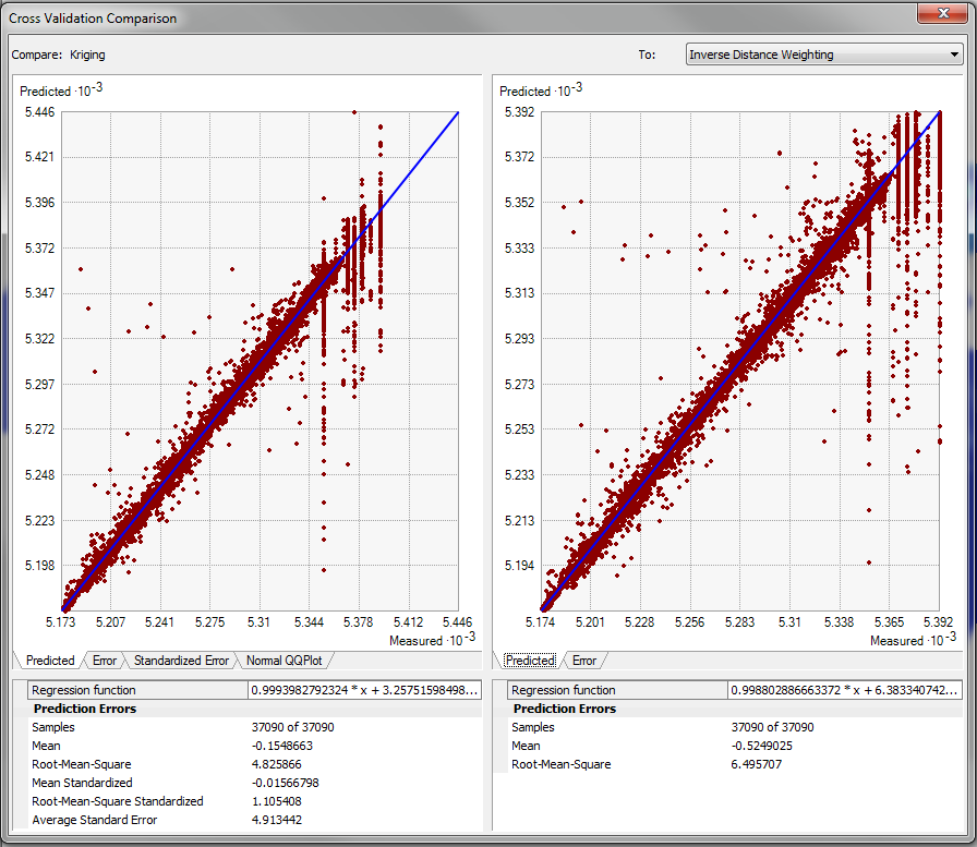
The "Validation/Prediction" option opens the "GA Layer to Points" tool, tests observed location points against the producted surface. The output of the tool provides a feature layer that includes predicted values, error, standard error etc in its attribute table. We can summarize the error, and compare:

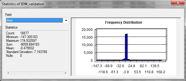
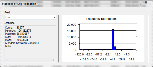
In this case, mean error is lower for Kriging!