Statistical Analysis
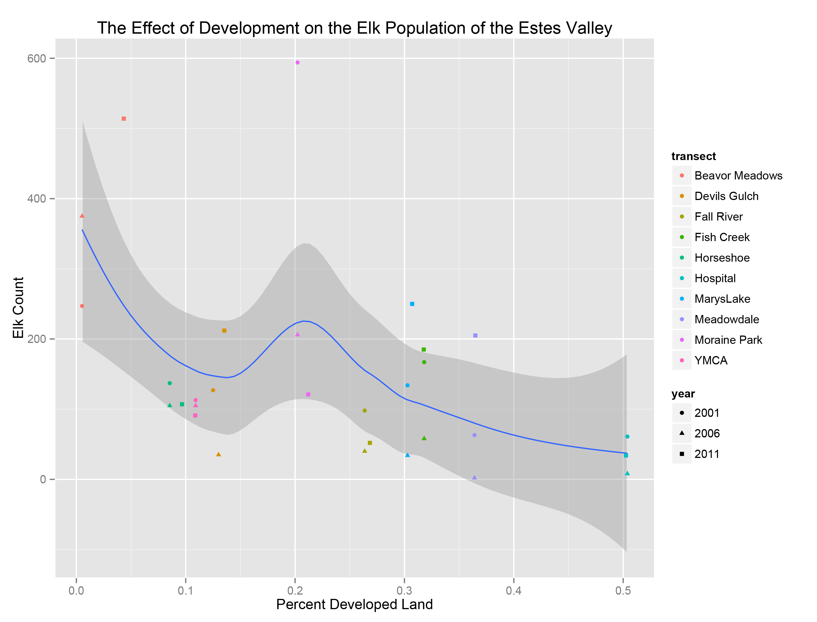
The following graph shows the number of elk counted versus the percent of developed land by transect (shown in different colors) and year (shown in different shapes). The curve and resulting confidence interval are the result of fitting a loess smoother function to the data. As we can see, the data do appear to have a negative relationship with regards to elk population within a region and the percent development, i.e. the higher the development, the lower the elk count.
Modeling Approach:
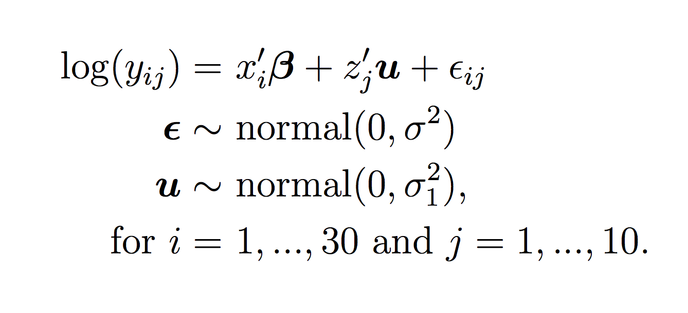
We used a generalized linear mixed model (Agresti, 2014), with a fixed effect for the percent of developed land (hereafter, developed), a fixed effect factor for year (year), and a random effect for transect (transect). Including the random effect for the transect indicates that we expect dependence within the same spatial regions on a local scale. In other words, the elk are likely to be found in areas where they have been found before, i.e. there is spatial dependence. It is arguable that the years during which the elk were surveyed could also have temporal dependence, but since the years of surveying were so dispersed (with 5 year intervals) we believe that these could be treated independently. A finer scale analysis with single year to year spatial and temporal dependence could be an interesting extension of this analysis.
The following formula shows the general form of the model:
Model Fitting:
The model was approximated in R using the lme4 software package (Bates et al, 2014). Because of the small set of predictors in the model, the information criterion approach of multi-model inference was not used (Burnham and Anderson, 2002). Rather, we fit the model which ultimately represented our understanding of the system as described above (Verhoef, 2014).
The following table shows the variables and type that were used in the analysis.
| Variable | Type | Fixed/Random Effect |
|---|---|---|
| Elk Count (y) | Response | - |
| Developed | Predictor | Fixed |
| Year | Predictor | Fixed |
| Transect | Predictor | Random |
Data for the percent development extracted from the NLCD dataset:
| Transect Name | Year | Percent Development |
| Beavor Meadows | 2001 | 0.00519 |
| Beavor Meadows | 2006 | 0.00519 |
| Beavor Meadows | 2011 | 0.04335 |
| Devils Gulch | 2001 | 0.12507 |
| Devils Gulch | 2006 | 0.13002 |
| Devils Gulch | 2011 | 0.13528 |
| Fall River | 2001 | 0.26364 |
| Fall River | 2006 | 0.26364 |
| Fall River | 2011 | 0.26839 |
| Fish Creek | 2001 | 0.31803 |
| Fish Creek | 2006 | 0.31803 |
| Fish Creek | 2011 | 0.31766 |
| Horseshoe | 2001 | 0.08539 |
| Horseshoe | 2006 | 0.08539 |
| Horseshoe | 2011 | 0.09661 |
| Hospital | 2001 | 0.50387 |
| Hospital | 2006 | 0.50387 |
| Hospital | 2011 | 0.50258 |
| Meadowdale | 2001 | 0.36408 |
| Meadowdale | 2006 | 0.36408 |
| Meadowdale | 2011 | 0.36486 |
| MarysLake | 2001 | 0.30278 |
| MarysLake | 2006 | 0.30278 |
| MarysLake | 2011 | 0.30706 |
| Moraine Park | 2001 | 0.20227 |
| Moraine Park | 2006 | 0.20227 |
| Moraine Park | 2011 | 0.21202 |
| YMCA | 2001 | 0.10905 |
| YMCA | 2006 | 0.10905 |
| YMCA | 2011 | 0.10868 |
See the results page for model output and summary.
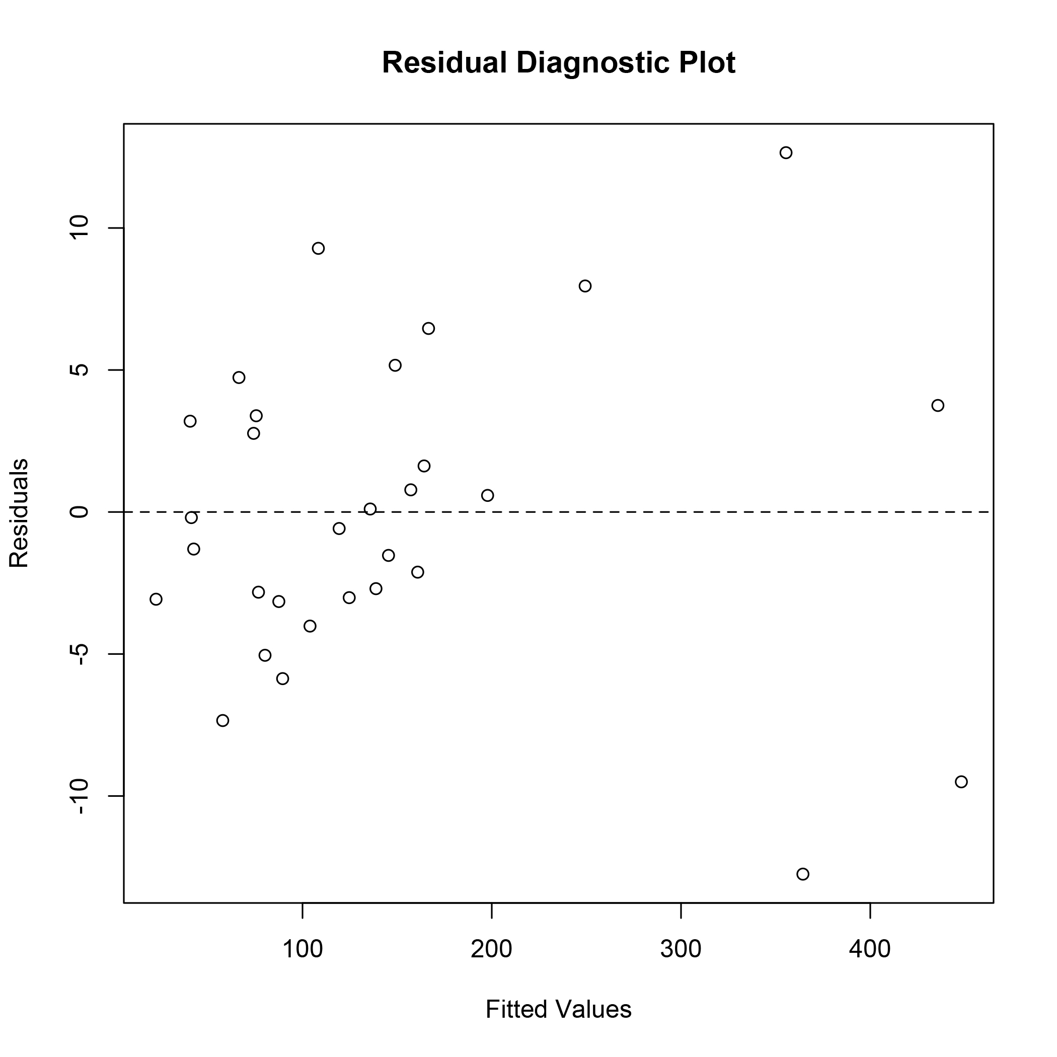
Diagnostics:
High variability of the response variable led to relatively wide confidence intervals. However, standard diagnostics did not reveal any heteroskedasticity or violations of independence. The following plot of the residuals shows no issues with the model fit, except for the high variability as seen in the range of the residual values. A chi-square test for over-dispersion was statistically significant (Χ2 = 36.93, p < 0.0001). This indicates that the assumption of equal moments for the Poisson distribution is violated. This is not uncommon for data arriving from processes observed in nature. A zero-inflated Poisson may provide a better fit to this data but was not explored in this analysis.