ArcGIS Concepts
Digitizing Driving Transect Rasters
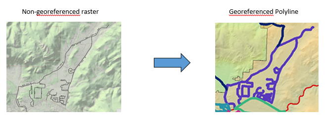
The first step in our analysis involved digitizing maps that were provided by the National Park Service. The ArcGIS expert at the park was unavailable at the beginning of this project so we attempted to digitize the driving maps which are usually provided to the volunteers during surveys.
To digitize the maps, the first step in this intricate process involved using an extremely helpful tool called the Georeferencing Tool. This tool allowed us to upload a non-georeferenced jpeg picture as a raster, and “snap” it to a spatially referenced location (Estes Park, CO) using a series of control points (road intersections). We snapped images for 7 different jpeg maps before receiving an e-mail from the Park Service ArcGIS expert with all the digitized routes we needed within a shapefile, which included 10 routes.
Buffering Driving Transects
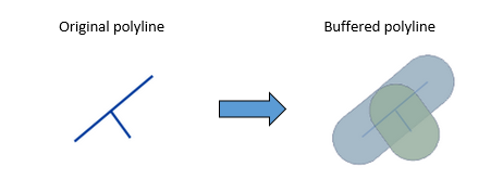
We decided that we needed to conduct our spatial analyses on an area surrounding the polylines where the elk were viewed. Each polyline on the map represents a driving transect (road) where employees and volunteers with Rocky Mountain National Park observed and counted elk. We estimated that the maximum distance at which people could view elk from the roads (taking vegetation into account) would be approximately 500 meters. The buffer tool created a polygon buffered 500 meters around the driving transects. For example:
Kernal Density Estimation
The Kernel Density Tool calculates the density (magnitude per unit area) of certain features, including points or polyline. Each buffered polyline on the map is associated with a number of elk, as is displayed in the following example attribute table:
| Elk Route | Elk Count |
|---|---|
| Devils Gulch | 355 |
We then ran the Kernel Density Tool for all the driving transects (buffered polylines) to get the probability density function for the number of elk within a square kilometer across the study area in the Estes Valley, CO.
National Land Cover Database Data
What is it?
The National Landcover Database (NLCD) uses the Normalized Difference Vegetation Index (NDVI) to detect changes in vegetation by measuring the difference in light reflected by plants. More specifically, green vegetation (that is photosynthesizing) reflects near-infrared light, and the more leaves a plant has, the more intensely this will be reflected. Near-infrared light is not within human’s visible spectrum of light, which is partly why they appear green.
The NDVI is a formula that measures the difference between near infrared light reflected minus the visible light reflected divided by the total of the two. The resulting ratio provides an index for determining the amount of vegetation in an area, such that values closer to +1 indicate larger amounts of green vegetation, while values closer to -1 indicate vegetation that is changing color due to season, disease, or just dying in general (zero means no vegetation). Scientists can compare ratios for the same area to see how vegetation has changed over time.
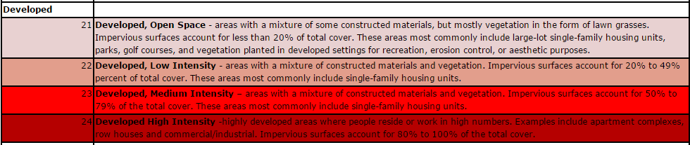
The NLCD also provides a legend to let users know what certain colors mean. We were mainly concerned with anything pertaining to development, which was classified as follows:
Adding elk exclosures to the NLCD
The National Park Service constructed elk exclosure in 2008, which we wanted to add to the NLCD data for the 2011 map as "Developed Open Space". First, we converted polygons of elk exclosures into rasters using the Polygon to Raster Tool. We then used the Clip Tool to trim the NLCD data to the Study Area boundary (Rocky Mountain National Park plus the Estes Park city limit). The Extract by Mask Tool allowed us to extract NLCD data to place into the exclosure raster (the mask we set). Once the NLCD data was included in the exclosure raster, we used the Reclassify Tool to reclassify the newly added NLCD data in the exclosure as "Developed Open Space". The Raster Calculator provided the means for adding the newly classified exclosure raster with the NLCD raster to create a new raster with the NLCD data combined with the newly designated "Developed Open Space" for the elk exclosures.
Reclassifying and clipping NLCD data
We used the Reclassify Tool for the NLCD data (clipped to the study area), such that all the data was reclassified as either "Developed" or "Not Developed" land. We also used the Clip Tool to trim the reclassified NLCD raster to match the extent of each buffered driving transect (buffered to 500 m). Since each driving transect contained its own reclassified NLCD data, we could see how much development was associated with each transect in 2001, 2006, and 2011. This information was used for a Generalized Linear Mixed Model to see if there were changes in the number of elk by transect based on the amount of development in 2001, 2006, and 2011.