GIS Analyses

PRISM Data:
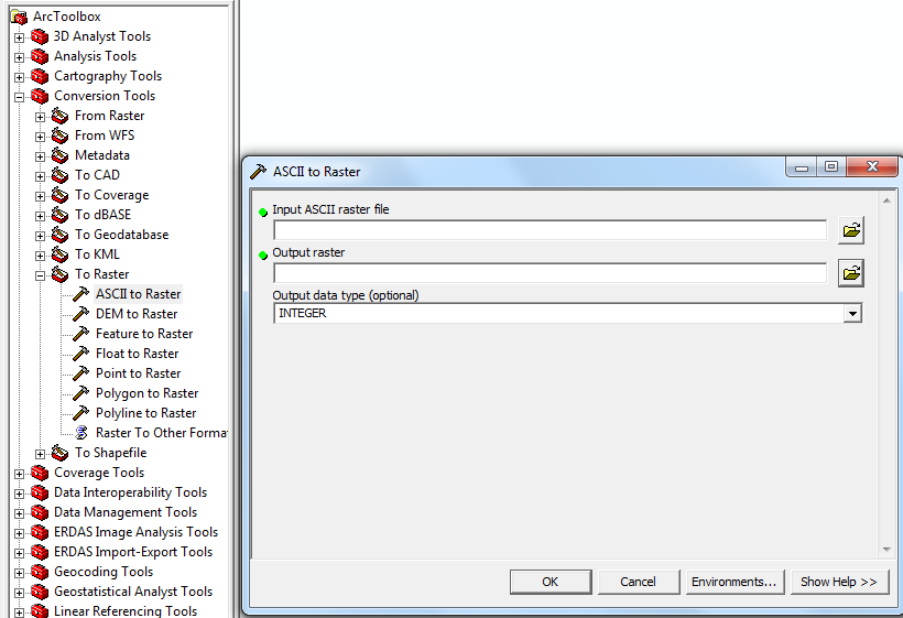
PRISM Data comes in a file with a name like us_tmax_2009.##, or us_ppt_1971_2000.##, where ## indicates the month (01-12).  The problem with this is that the average computer thinks that each file is a .01 or .02 file (etc).  So, the files were all renamed with an underscore replacing the period and a .txt at the end (us_tmax_2009_##.txt).  They were then turned into a raster on arcmap using the ascII to raster command:

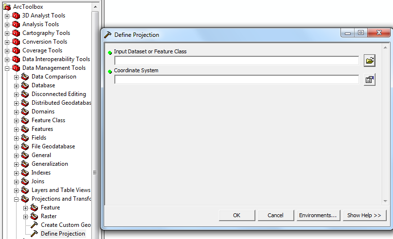
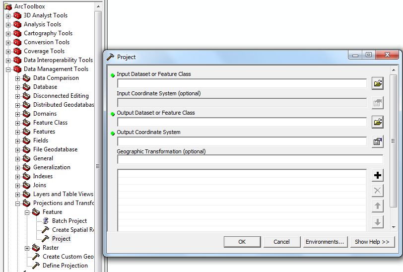
Once they were imported into ArcMap in the form of a raster file, a define projection was performed.

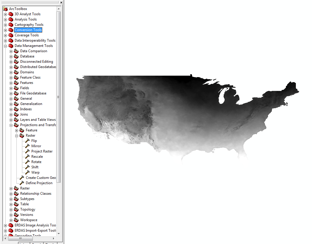
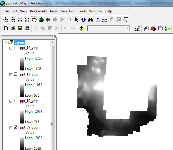
Then they were projected using Project Raster.  PRISM gives data in the form of a raster of the entire United States:

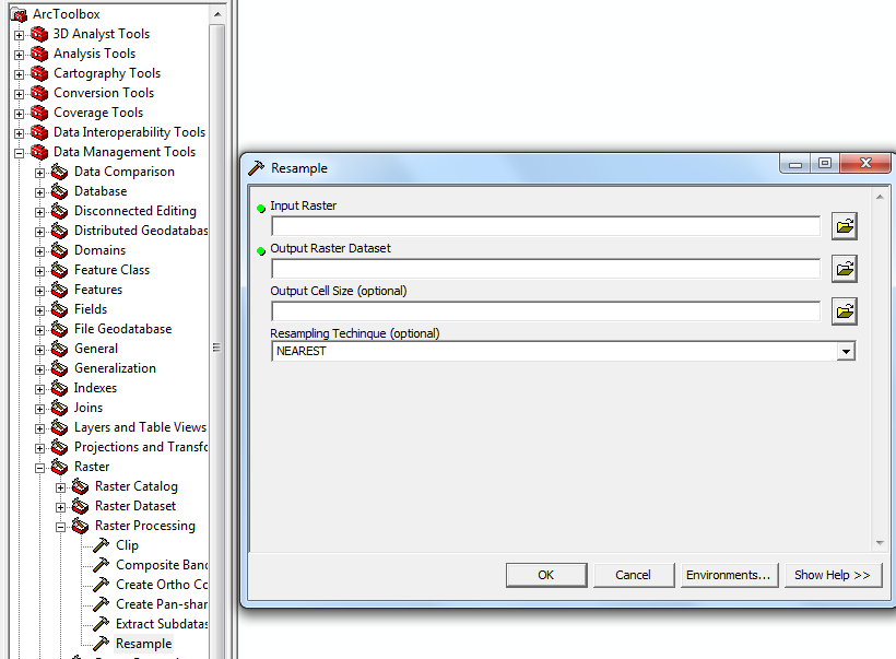
Because the PRISM data has very low resolution, it must be resampled to the same resolution as one of the rasters that came about from kriging the weather station data.  So, it must be resampled with the “resample” tool, and the output cell size is selected by clicking the folder on the right and importing one of the krigged rasters.

The data must then be clipped using the raster calculator on the spatial analyst tool.  To do this, spatial analyst was activated, then the spatial analyst toolbox was brought up.  The analysis mask and extent were both set to the YPG Boundary, which is appropriately named.  Then, using the raster calculator, a new name is given to the new raster, and the prism rasters are born.

 

 

YPG Data:

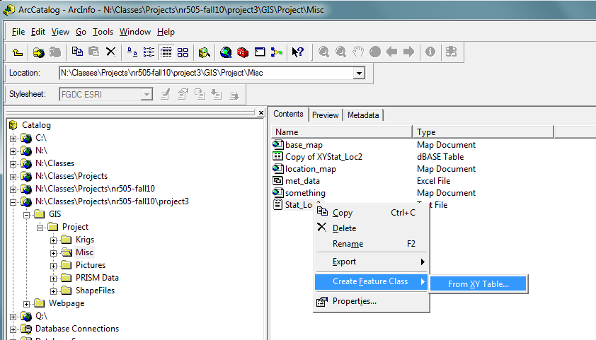
To create the weather station shape file, a .txt file was created with the latitude and longitude coordinates written down for each station.  To turn them into a shape file, ArcCatalog was opened, the file was located, and after right clicking and “create feature class” was selected, then “from XY table.”  Then the file was turned into a shape file with points on it.

Next, the precipitation and maximum temperature data was entered manually into the "xy_statloc" shapefile. Then, The datum was defined using define projection, then it was projected using project, under data management. 

To create a raster by kriging, Spatial Analyst is once again used.  From the Spatial Analyst toolbar, the “interpolate to raster” option was selected, then “kriging.”

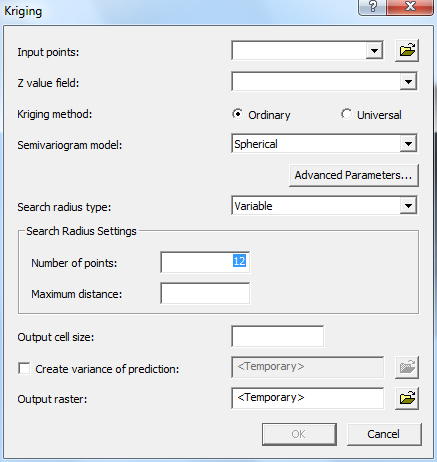
All the defaults were used, except for the average precipitation data for April and May. For more information on that, see the GIS Concepts page. The krig creates a square raster that encompasses all of YPG. To get only YPG, a new, clipped raster was made with Raster Calculator using the method described above.

 

 

PRISM and YPG Data:

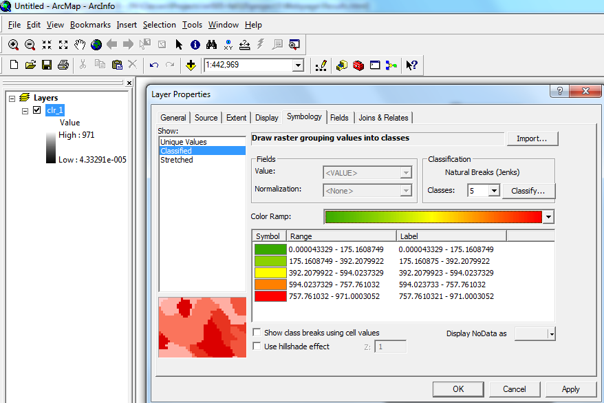
To get the colored maps, one raster (called clr_1 for precipitation data and clr for max temperature data) was created from one of the other rasters, and using map algebra and the raster calculator, this raster was made to have pixels whose values ranged from the lowest value out of all 12 months to the highest value out of all 12 months. After right clicking and selecting properties and going to the symbology tab, a then clicking “classified,” a classification system was created for this dummy raster, and then imported into all of the other rasters. It is in this way that all the pictures in the results section are rated using the same rating system for precipitation and maximum temperature.