GIS Concepts

This project incoorperates several basic GIS concepts: database managment, data type selection, data manipulation, measurement, and optimization. Two sources of data were used for this project: survey coordinates obtained with a GPS and a digital elevation model (DEM) obtained from satelite. All of the following GIS concepts were used to reach our project goal of determining a least cost path.

Single click on images to reduce size. Double click to enlarge.

Database Management: A personal geodatabase was used to organize all data set types (i.e., feature classes, raster data sets) used in the analysis. The advantages of using a personal geodatabase is consistent coordinate systems, topologies, raster catalogs, etc. Using a database also reduces problems associated with data transfer between group members.

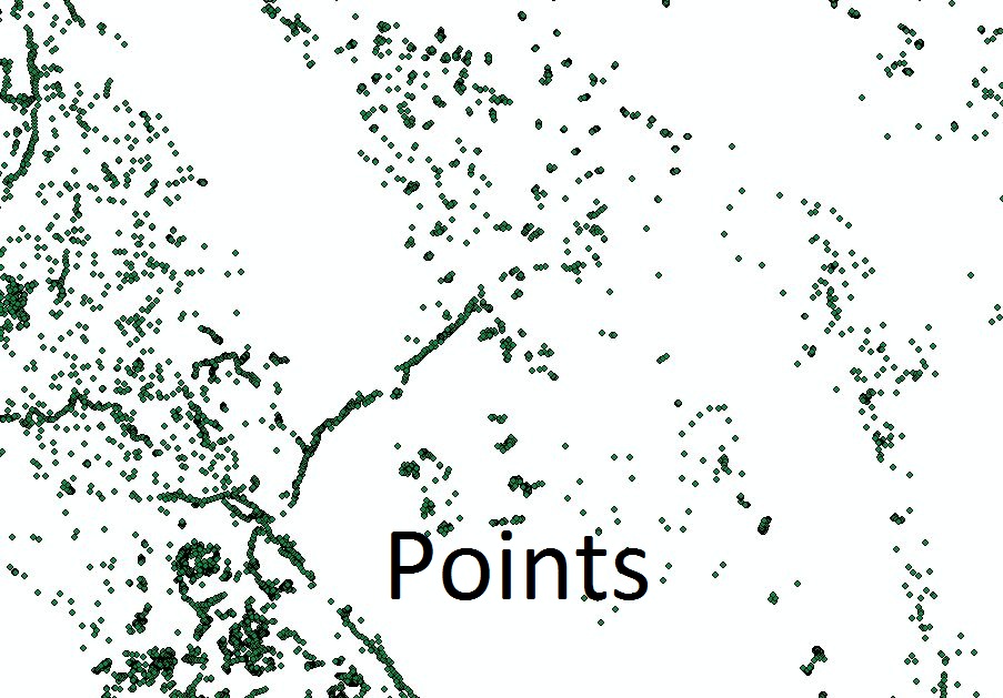
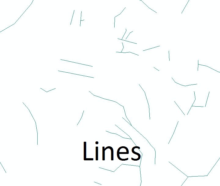
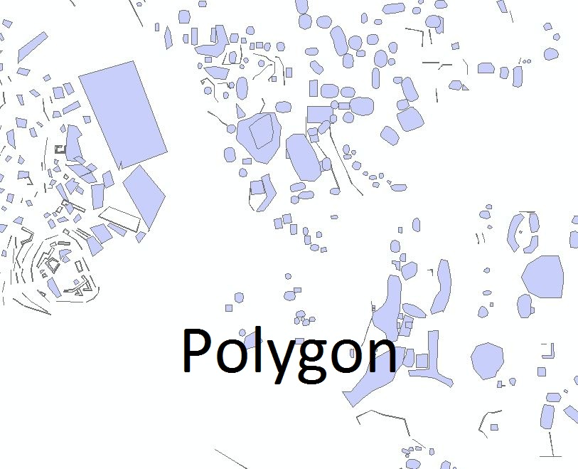
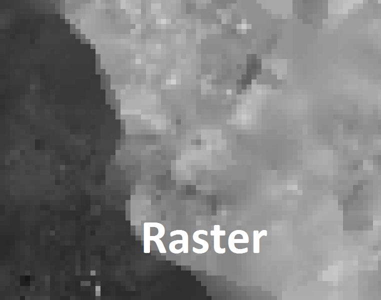
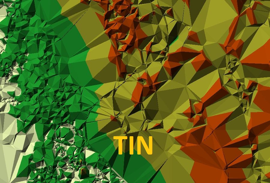
Data Type: Data from a GIS can be represented in several ways in ArcMap. There are 3 main feature classes used to represent point and vector data (i.e., points, lines , polygons). Continuous data can be represented with rasters, which are blocks of cells where location attributes are stored at the cell resolution such that any location within the cell is represented by the cell value. A triangulated irregular network (TIN) can also be used. The vertices of the triangles represent known values, those values are then used to make calculations for the values of regions between points. TINs are commonly used for surface representation where each point or triangle vertex is a known elevation. The choice of how to represent the data will be determined by the appropriate analysis method chosen to answer the question.

Single click on images to reduce size. Double click to enlarge.

Resolution: A key concept when working with rasters is the resolution of the data. A finer resolution raster will have more information in the form of smaller cell sizes allowing for representation of variation across smaller distances. A finer resolution raster will more accurately represents reality at the expense of requiring more information. An appropriate resolution should be determined for the question being asked.

Data Manipulation There is often a multi step process between data collection in the field the end of an analysis (see flowchart). We used the following to manipulate our data:

Projection- A key concept in geography is the representation of a sphere on a flat surface. A projection is a mathematical transformation from spherical coordinates to a planer coordinate system. One key idea to remember is that all projections have distortion in one or all of the categories: distance, shape, area, or proximity. The appropriate projection should be determined by the purpose of the represented information.

Change in Data Type- Data can be converted back and forth between different types of feature classes (i.e., point to polygon, point to line) or even from a feature class to a raster data set (e.g., polygon to raster, point to TIN).

Select by Attribute- A query used to select records based on attributes. This is a key idea for organizing and grouping data.

Classification- A key part of science is classification of information into meaningful categories. This grouping allows for sorting and summarizing of unique units allowing for a potential of generalization and possibly pattern recognition. Depending on information collected, data can be represented using nominal, ordinal, interval and ratio formats.

Raster- There are many calculations that can be performed on a raster to develop new rasters. A DEM or raster containing elevation data is used to calculate rasters for slope and aspect.

Slope Raster- (Maximum Change in Elevation between cell of interests and neighbor cells)/(Cell width)

Cost Distance Raster- Given source cells and a cost raster, the minimum cost required to reach a given cell from any source cell is assigned to the cell of interest.

Back Link Raster- Cells surrounding a given cell are numbered 1-8. The cell of interest is assigned the number from the cell that is the lowest cost back to any source cell.

Least Cost Path Raster- A set of cells that delineate the most cost effective path across a cost raster.

Dissolve- Combining multiple feature class records of like type into a single record.

Single click on images to reduce size. Double click to enlarge.

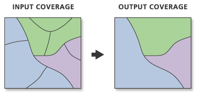
graphic source: esri online help

Clip- Can be used to cut out areas of interest. The clip keeps area within set of polygons or the area outside a set of polygons.

Single click on images to reduce size. Double click to enlarge.

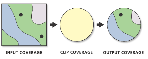
graphic source: esri online help

Merge- is used to combine data of like type from different input sources into a single feature class.

Single click on images to reduce size. Double click to enlarge.

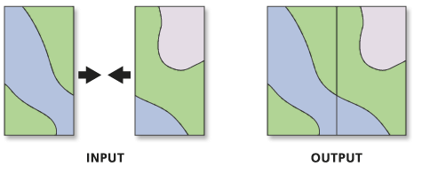
graphic source: esri online help

Digitization- in some cases information will need to be manually created in ArcMap. Heads up digitization can be used to create layers manually. In our case we digitized social boundaries using expert knowledge.

Resample- A raster can be resampled to form a "smoother" rasters with smaller cell sizes by interpolating values for the smaller cells from the original raster. We used a cubic polynomial to smooth our original 4 m raster to form a .5 m raster. Interpolation needs to be done with caution as the new values may not reflect true variation across the smaller cells.

Single click on images to reduce size. Double click to enlarge.

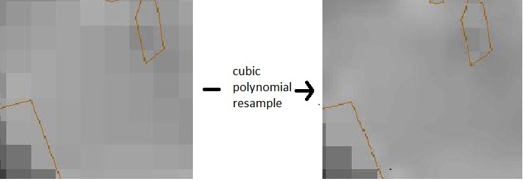Figure: Non-resampled raster (left) vs. resampled using a cubic polynomial fit to a 4 m DEM in order to create a .5 m smooth DEM.

Reclassify- raster values can be grouped or reassigned new values.

Optimization:

Path Distance- Using a DEM cost associated with crossing each cell within a raster can be calculated. The cost may vary depending on the direction a cell is crossed (e.g., traversing or crossing a cell where adjacent cells are of similar elevation in one direction as opposed to crossing a cell where adjacent cells are of different elevation.)

Single click on images to reduce size. Double click to enlarge.

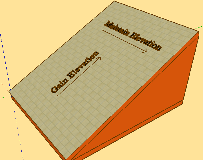
graphic source: David Lewis created in Google Sketchup ver: 7.1.6860

back-link- raster created to keep track of direction back to least cost source cell. Dirctions are limited to 8 values each of which represents one of the surrounding cells.

least cost path- least cost path from the least cost distance and back link raster.

Single click on images to reduce size. Double click to enlarge.

Graphic sources: (left) esri online help. (right) David Lewis created in Google Sketchup ver: 7.1.6860

Free JavaScripts provided
by The JavaScript Source