Introduction
Location Map
Base Map
Database Schema
Conventions
GIS Analyses
Flowchart
GIS Concepts
Results
Conclusion
References

GIS Analyses

GIS Analyses

Field Sampling Protocol:

Our analysis looks in particular at two landscapes owned and operated by Boulder County Parks and Open Space, Hall and Heil Valley Ranches in the north-central foothills of the Front Range. These 14 study plots are each 0.5 hectare in area. Within each 0.5 hectare study plot, there are 4 subplots of 12.7 meter radius. Within these 12.7 meter radius subplots, all live trees, dead trees, and remnant stump, log, and snag material were sampled using increment boring or chainsaw sampling for further dendrochronological cross-dating to occur in the laboratory. In addition to sampling for age, all trees and remnant material were sampled and measured to get spatial location on site and size of material. These sub-plots (12.7m) were then extrapolated onto each larger quadrant, where all trees and remnant material that was classified as ‘old’ (establishment date of pre-1860) were measured. In addition to these measurements, all evidence of fire-scars on live and dead trees and remnant materials were sampled and cross-dated in the laboratory. The locations of all sampled and stem-mapped trees and remnant materials were all converted to utm coordinates for further spatial analysis.

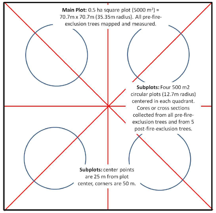
photo credit: Colorado Forest Restoration Institute & USFS- Rocky Mountian Research Station

The stump in this photo provides an example of a remnant sample which was sampled and cross-dated to obtain fire history of the sample sites. The stump was also mapped spatially to obtain detailed stand spatial reconstruction.

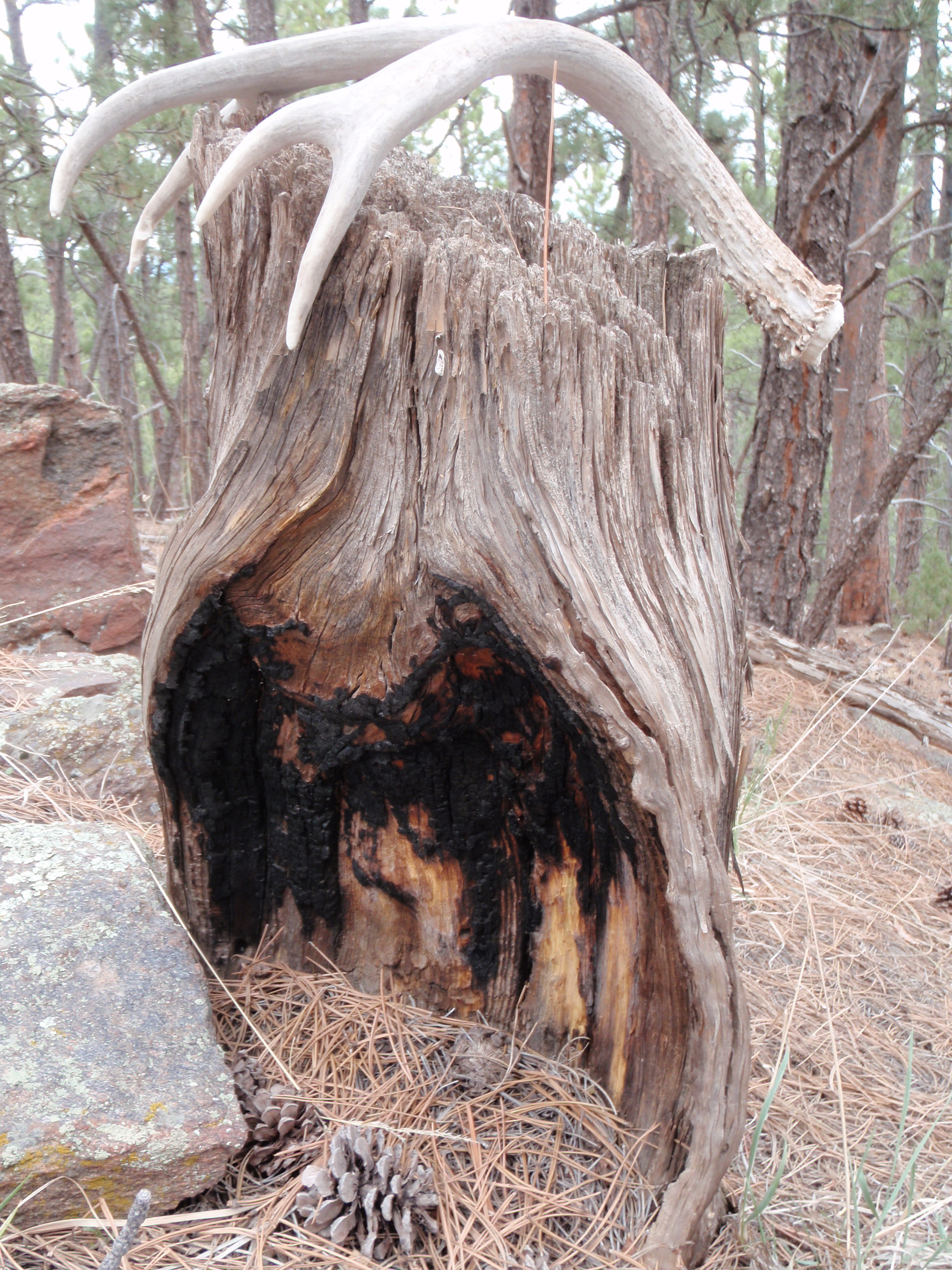
photo credit: Colorado Forest Restoration Institute & USFS- Rocky Mountian Research Station

Landscape Data Preparation:

The ranch property boundaries and access roads shapefile were acquired from Boulder County Parks and Open Space (BCPOS) officials (OS_COUNTY_OPEN_SPACE.shp). The overall property boundary file contained boundaries for all Boulder County Open Space areas, so the Select By Attributes tool was utilized to create individual shapefiles for each Hall and Heil Valley Ranch boundaries (HA_Boundary.shp and HE_Boundary.shp, respectively). Each of these boundary shapefiles were then used to clip our study sites to produce HA_StudyPlots.shp- Shapefile of study plots within the Hall Ranch Boundaries, HE_StudyPlots.shp- Shapefile of study plots within the Heil Valley Ranch boundaries, and StudyPlots_Clip.shp- Shapefile of study plots clipped to Hall and Heil Valley Ranch boundaries.

The files that contained the data for the roads within the property boundaries came from two sources: US Census Bureau and BCPOS. These two files were merged using the Merge tool, resulting in the HallHeilRdsFinal.shp file.

The data for the streams within the property boundaries came from a previous lab excercise in the NR 505 course, and was originally downloaded from the USGS server. This STREAMS.shp file was clipped to each property boundary to create streams shapefiles for each property (HA_Streams_clip.shp and HE_Streams_clip.shp).

Density Analysis Data Preparation:

The master Excel file developed from the Colorado Forest Restoration Institute and the Rocky Mountain Research Station contained plot level data for areas located throughout the Colorado Front Range. For this GIS analysis, we are only concerned with the plot data for Hall and Heil Valley Ranches. Once this data was extracted from the master file, it was imported to ArcGIS for further management and analysis.

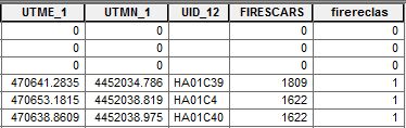
The master Excel file contained information for all trees on the plot, and UTM locations and dates of fires for each fire scar that was analyzed. Although the master file did contain information on fire scar dates for the plot level data, the format of this information was incompatible with ArcGIS. In order to make this information more usable, a separate Excel file was created based off of the UID (plot name), and the fire scar dates were manually added in association with each plot's UID.

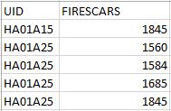
This Excel file was then joined with the master file based off of UID, creating the HA_HE_TotalFireScar.shp file. Within this file in ArcGIS, a new field was added to the attribute table using the field calculator to assign a value of "1" to any plots that had a fire scar date that was greater than "1". This allowed for the kernel density tool to analyze the density of fires based off of the amount of individual fire years.

In order to understand how many fires occurred in the pre-settlement era in comparison to the post-settlement era, each fire year was manually recorded for each study site. Each individual recorded fire year that occured was tallied and divided into which property the fire was recorded in, and no duplicates were recorded in the same property. This allowed for an accurate count of the number of fire years that were recorded for each property for both the pre- and post-settlement eras.

Canopy Area Data Preparation:

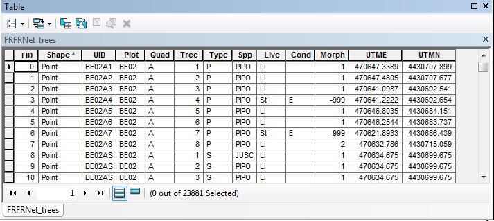
The master Excel file utm coordinates were imported into ArcGIS and used to develop the FRFNET_trees.shp- Shapefile of all the utm coordinates of live trees and remnant material within all Front Range study plots. This shapefile contained all tree and remnant information for all plots, which consisted of utm location, age (morphology), condition, status, and any other pertinent information.

This FRFNET_trees shapefile was then ready for analysis, which is depicted in its respective flowchart.

Cost Analysis Data Preparation:

To perform a cost analysis of our study areas, we needed needed to obtain a digital elevation model and mask it to our overall study area. We obtained the DEM from the usgs national map view database. The process we used to prepare our DEM is depicted in its respective flowchart.

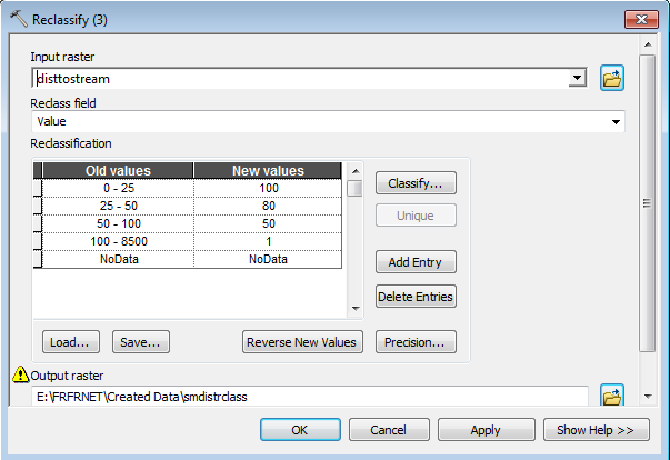
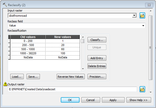
We used the finished DEM file, hallheildem, HallHeilRdsFinal, and ha_he_steams_clip files to perform the cost analysis of our study areas. In order to perform this analysis we needed to conduct three seperate reclassifications of each of these files after using tools to designate the three costs which will be weighed in each cost. These three costs were identified as: distance from roads, percent slope plots are located on, distance from stream. The step-by-step process is depicted in its respective flowchart. A composite cost-distance shapefile, costsurfacefinal.img- Raster dataset calculated using Raster Calculator tool summing the roadscost, slope_reclass, and smdistrclass shapefiles, was used to develop a final map integrating all three landscape variable costs to treatment.

Depicted below are the reclassification values given to each of the three categories:

Slope-Cost

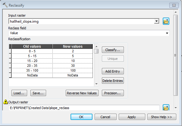
Note: A slope of 35% was identified as the maximum threshold mechanical treatments could be performed on.

Distance-from-roads Cost

Distance from Stream-Cost