
Introduction
Location Map
Base Map
Database Schema
Conventions
GIS Analyses
Flowchart
GIS Concepts
Results
Conclusion
References
GIS Analyses
Vector GIS Analyses
Screen capture of the process of querying stands for designation of priority and management strategy.

Click on Image to Enlarge
Stands are selected first by identifying roads or trails of a specific maintenance level and selecting individual stands that intersect them. The select by location tool also has a useful option where a buffer can be added for selecting any stands that are close enough to that particular road. From this selection we then identify the stands with mean slopes that correspond to the different management actions by using the select by attributes tool and manually entering in the appropriate attributes for each feature.
Management Action Matrix |
|||||
Stand Access |
Class |
Priority |
Mean Slope |
||
< 25% |
25% - 35% |
> 35% |
|||
Roads |
5 |
1 |
Mechanical |
Hand Treat Stand |
Treat Buffer Zone |
4 |
2 |
Mechanical |
Hand Treat Stand |
Treat Buffer Zone |
|
3 |
3 |
Mechanical |
Hand Treat Stand |
Treat Buffer Zone |
|
2 & 1 |
4 |
Mechanical |
Hand Treat Stand |
Treat Buffer Zone |
|
Rec Sites |
All |
1 |
Mechanical |
Hand Treat Stand |
Treat Buffer Zone |
Trails Only |
5 |
1 |
Hand Treat Buffer Zone Only |
||
4 |
2 |
||||
3 |
3 |
||||
2 & 1 |
4 |
||||
Screen capture of the attribute table for final treatment stands joined with the Zstat output table.
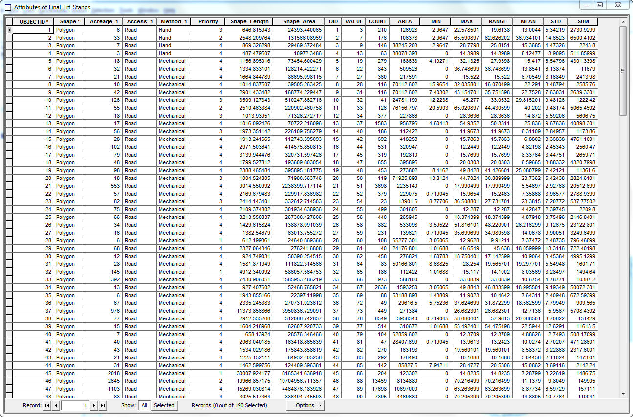
Click on Image to Enlarge
Raster GIS Analyses
Part 1: Management Importance
UNF land managers must consider the impacts of SAD on the many uses of the UNF. For our purposes, management importance will be a function of recreation safety & roadways management, aesthetics, and ecological value. Maps of SAD affected stands are available for the Region II: Rocky Mountain Region Aerial Detection Survey (USDA FS 2010). These stands were mapped by means of digitizing stands during aerial survey. The three different management importance categories represent different objectives of land managers. These objectives can be met by different management practices. For example, a stand that is intersected by a road, does not all have to be treated. Only an area within a given buffer distance must be treated. Similarly, stands that span viewsheds need not be considered an inseparable unit. For this reason, Part 1 of the raster analysis will evaluate the landscape at the level of a pixel.
Management Importance Categories |
Point value |
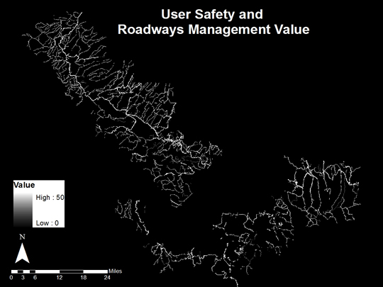
User safety and roadways management value |
0-50 |
Aesthetic Value |
0-25 |
Ecological Value |
0-25 |
National forest land managers must be concerned with the safety of national forest users at recreation sites, on trails, and on roads within the national forest. SAD affected stands have high densities of large dead trees that can be hazardous to users. Dead trees that fall over trails and roadways can also cause travel difficulties. The eventual cost of removal of fallen trees that block trails and roads is further motivation for pre-emptive management. Portions of trails and roads that intersect or fall within close proximity of SAD affected stands can be managed by means of removing dead trees within a buffer distance. The Prescott National Forest (USDA FS 2010) has suggested buffer distances of 100ft for trails and 200ft for roads for removal of mountain pine beetle-killed trees. We calculated the strait line distance from recreation sites, roads, and trails for a 25x25m raster grid of the study site and then reclassed the distance grids with thresholds based on the buffer distances in the following table using conditional statements in raster calculator.
Features |
Buffer Distance |
Point value |
Recreation sites – Point shapefile |
400ft |
50 |
Roads – Polyline shapefile |
|
|
5 – High degree of user comfort |
200ft |
50 |
4 – Moderate degree of user comfort |
200ft |
40 |
3 – Suitable for Passenger Cars |
200ft |
30 |
2 – High Clearance Vehicles |
100ft |
20 |
1 – Basic Custodial Care (Closed) |
100ft |
10 |
Trails – Polyline shapefile |
|
|
TC5 – Fully developed |
100ft |
50 |
TC4 – Highly developed |
100ft |
40 |
TC3 – Developed |
100ft |
30 |
TC2 – Moderately developed |
100ft |
20 |
TC1 – Minimally developed |
100ft |
10 |
Code examples used in raster calculator:
recsitebuff = con([recsitedist] < 121.92, 1, 0)
tc1binbuff = con([tc1traildist] < 30.48, 1, 0)
c1roadbuff2 = con([c1roadbuff] < 30.48, 1, 0)
Raster calculator was then used to...
(Below are EXAMPLES of code used)
... multiply the binary buffers by their respective point values from the table above.
precsitebuff = [recsitebuff] * 50
ptc1binbuff = [tc1binbuff] * 10
pc1roadbuff = [c1roadbuff2] * 10
...sum the component points values
pbufftotal = [precsitebuff] + [ptc1binbuff] + [ptc2binbuff] + [ptc3binbuff] + [ptc4binbuff] + [ptc5binbuff] + [pc1roadbuff] + [pc2roadbuff] + [pc3roadbuff] + [pc4roadbuff] + [pc5roadbuff]
...trim the total value to a max of 50
pbufftotal_tr = con(pbufftotal > 50, 50, pbufftotal)
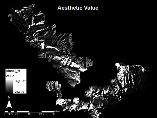
Aspen viewing is important to the economy of southwest Colorado. Our assumption is that tourists use national forest land for aspen viewing by means of recreation sites, roads, and trails. Furthermore, they preferentially favor views from recreation sites and from more developed roads and trails. We calculated viewsheds from the following point and polyline features for the entire UNF using the Aster DEM as the terrain surface. This resulted in approximately 25x25m grids with values indicating whether each pixel on the landscape is visible or non-visible. The output grid also has a real integer value representing the number of points or polyline vertices that could see that pixel on the landscape. The maximum grid value was used to divide the viewshed grid in order to create an index from 0-1 using raster calculator.
Example code:
recsites = [recsites_fl] / 8
c1road = [c1road_fl] / 4199
tc1trail = [tc1trail_fl] / 1154
Features |
Point value |
Recreation sites – Point shapefile |
25 |
Roads – Polyline shapefile |
|
5 – High degree of user comfort |
25 |
4 – Moderate degree of user comfort |
20 |
3 – Suitable for Passenger Cars |
15 |
2 – High Clearance Vehicles |
10 |
1 – Basic Custodial Care (Closed) |
5 |
Trails – Polyline shapefile |
|
TC5 – Fully developed |
25 |
TC4 – Highly developed |
20 |
TC3 – Developed |
15 |
TC2 – Moderately developed |
10 |
TC1 – Minimally developed |
5 |
Raster calculator was then used to...
(Below are EXAMPLES of code used)
... multiply the indexed viewshed values by their respective point values from the table above.
precsites = [recsites] * 25
pc1road = [c1road] * 5
ptc1tr = [tc1trail] * 5
...sum the component points values
ptotal = [precsites] + [pc1road] + [pc2road] + [pc3road] + [pc4road] + [pc5road] + [ptc1tr] + [ptc2tr] + [ptc3tr] + [ptc4tr] + [ptc5tr]
...trim the total value to a max of 25
ptotal_tr = con(ptotal > 25, 25, ptotal)
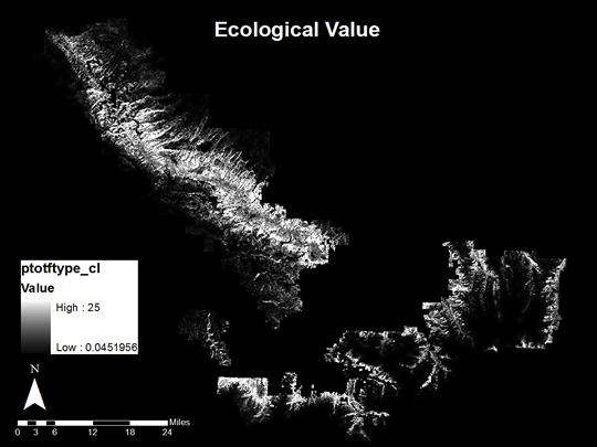
The ecological value of impacted stands can be assessed by means of the actual vegetative cover of those areas digitized as being affected by SAD. Sketch mapping is not an exact or error-free procedure. There may also be SAD induced aspen mortality in forests that have only a small portion of aspen in them. An independent land-cover dataset that can address this issue is the Landfire current vegetative cover product. The current vegetative cover product is derived from Landsat, so it has a spatial resolution of 30x30m. The dataset was downloaded, reprojected, and resampled to match the rest of the raster datasets. Two current vegetative cover types include aspen: 2011 – Rocky Mountain Aspen Forest and Woodland and 2061 – Inter-Mountain Basins Aspen-Mixed Conifer Forest and Woodland. The 2011 type was prioritized because damage to pure aspen stands will have a more significant impact on the forest ecosystem than damage to mixed aspen conifer stands. Pixels within those classes were assigned values according to the table below. To account for the imperfection of remotely sensed classified products, small weights were also attributed to cells neighboring either of these forest types. This reduces the impact of misclassification and adds value to managing nearby stands.
Rasters |
Point value |
2011 – Rocky Mountain Aspen |
25 |
2061 - Mixed |
12.5 |
Indexed inverse-distance from 2011 |
5 |
Indexed inverse-distance from 2061 |
2.5 |
We used Spatial Analyst -> Distance -> Straight Line to create grids of distance from either vegetation cover type 2011 or 2061.
Then we used raster calculator...
(Below are EXAMPLES of code used)
... to invert the distance to GRIDs to create distance from GRIDs.
inv2011 = 1 / [dist2011]
...to rescale the GRIDs from 0-1.
index2011 = [inv2011] / 0.03956720232963562
...to multiply the compenent grids by the point values from the table above
distval2011 = [index2011] * 5
distval2061 = [index2061] * 2.5
...sum the component points values
ptotftype = [patch_2011] + [patch_2061] + [ft2011_float] + [ft2061_float]
...trim the total value to a max of 25
ptotftype_tr = con(ptotftype > 25, 25, ptotftype)
Resulting component value GRIDs were added together using Raster Calculator to get the final Management Importance Value GRID.
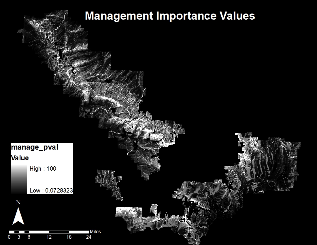
Click on Image to Enlarge
Part 2: Management Cost
Management costs vary based on terrain, which limits the management techniques that can be implemented, and the distance of management areas from access sites. Management techniques considered in this study include mechanical and hand felling/harvesting. Mechanical management techniques are preferred because they are quicker and require less human labor time. Hand management is less efficient. These management techniques are limited by terrain (slope) and access (distance from roads or trails). The management cost of a particular pixel will be determined as the sum of the terrain (50%) and access (50%) costs on a scale from 0 to 100.
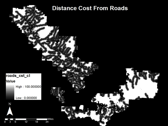
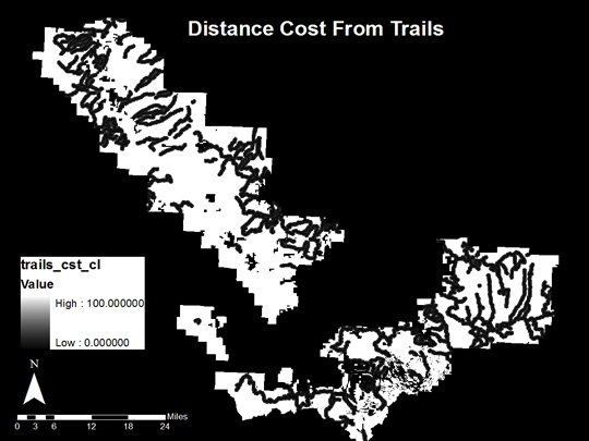
Access routes include roads and trails. Roads are easier access routes. Trails are more difficult access routes. To deal with this difference it is necessary to calculate distance rasters for both feature types and then to decide for each pixel, which distance to use. It is really only feasible to manage areas within 1000m of existing roadways without creating intensive new roadways. The road distance raster will be indexed from 0 to 1, with all distances greater than 1000m receiving an index value of 2 (to multiply out to 100 or maximum cost). It is assumed that trail access and trailside management is more difficult, since it must be done by hand. The trail distance raster was indexed from 0 to 1, with all distances greater than 500m receiving an index value of 2. These indexed distance rasters were then multiplied by the maximum distance point value of 50 (for 50%).
Rasters |
Point value |
Distance from roads (< 1000m) |
0-50 |
Distance from roads (> 1000m) |
100 |
Distance from trails (< 500m) |
0-50 |
Distance from trails (> 500m) |
100 |
Management technique implementation is determined by slope. Mechanical treatments are possible on slopes < 25%. Hand treatment is ideal on slopes from 25-35%. Hand treatment is possible, but expensive on slopes greater than 35%.
Percent slope |
Management |
Slope Index |
Point value |
< 25% |
Mechanical |
Percent slope / 25 |
10 + 10 * slope index |
25% ≤ slope < 35% |
Hand |
Percent slope / 25 |
20 + 20 * slope index |
35% ≤ |
Hand (difficult) |
NA |
50 |

The total management cost is the sum of the distance cost rasters and the slope-based management cost rasters. This total management cost was trimmed to 100 for the cases that were > 1000m from roads or > 500m from trails. At this point there are still two GRIDs: one with the distance cost from roads and one with the distance cost from trails.
The next step is to select those stands which have roads as their closest access points and those stands which have trails as their closest access points. This was accomplished in by means of zonal statistics with the zone file as the final I&D Aerial Survey Stands shapefile and the value raster as either the distance to roads or the distance to trails GRIDs. The outputs of these two processes were joined to the final I&D Aerial Survey Stands. Select by attributes was then used to select stands with smaller minimum distances to roads than minimum distances to trails or with minimum distances to roads equal to zero. The selection was then reversed to select those stands with smaller minimum distance to trails.
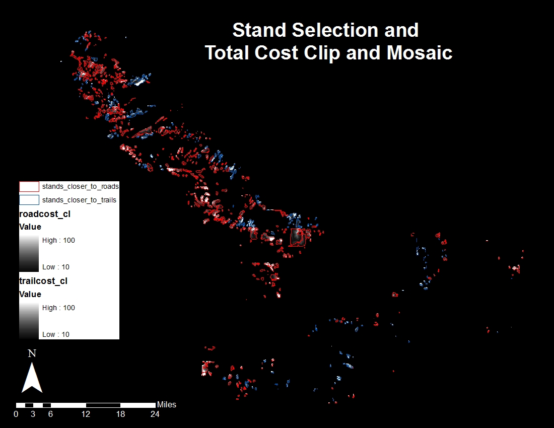
Click on Image to Enlarge
The total management cost raster with the distance cost from roads was then clipped to the extent of those stands closer to roads using Data Management -> Raster -> Raster Processing -> Clip with the clip to feature geometry option. The same was repeated for the total management cost with the distance cost from trails using the stands closer to road for the clip layer. The resulting GRIDs were then mosaicked using the Mosaic to new raster function.
The total management value raster was clipped to the extent of all SAD affected stands using Data Management -> Raster -> Raster Processing -> Clip with the clip to feature geometry option. The Value-Cost Difference raster was then created using raster calculator as the management value GRID minus the management cost GRID. Since management values and costs used in this project are not absolute values, the GRID subtraction operation resulted in many pixels with negative values. Our management values and management costs are really just relative scales. The management value system is based on a theoretical management plan and has no exact dollar value associated with the resulting benefit of management. We rescaled the Value-Cost Difference raster from 0-100 so that a uniform classification scheme could be applied to all rasters based on a score from 0-100.