
Introduction
Location Map
Base Map
Database Schema
Conventions
GIS Analyses
Flowchart
GIS Concepts
Results
Conclusion
References
Using GIS to Determine Native Felid Habitat in Urbanizing Areas and its Link to Human and Domestic Cat Conflicts
GIS Analysis
Our GIS Analysis has three major parts; data preparation and data analysis of question 1 and the data analysis of question 2. We willdiscuss the steps we took in all three parts.
Data Preparation:
County Parcels:
We collected shapefiles for all the private parcels in Montrose, Ouray, San Miguel and Boulder counties from each local county GIS office.
Project:
Once
we had the shapefiles we projected (Data Management Tools/Projections and Transformation/feature/Project) all of them to NAD 83 UTM 13N.
Select and Export:
After the parcels were projected we needed to determine a subset for our four study sites.
We selected all the parcels that met the following criteria and exported them as 8 separate files - Boulder Exurban, Boulder Urban, Montrose Exurban, Montrose Rural, Ouray Exurban Ouray Rural, San Miguel Exurban and San Miguel Rural.
Boulder Urban - parcels that were within 100 m
of natural areas, western side of Boulder
Boulder Exurban - in Boulder county but west of the city limits, surrounded by natural habitat
Uncompahgre Plateau Exurban - outside city limits
, less than 40 acres, surrounded by natural habitat
Uncompahgre Plateau Rural - outside city limits, greater than 40 acres
Once we had our acceptable parcels, we needed to narrow down our sample size further. In excel we imported the parcel numbers for all each of our four study sites: Boulder Exurban, Boulder Urban, Uncompahgre Exurban (Montrose, Ouray and San Miguel combined) and Uncompahgre Rural (Montrose, Ouray and San Miguel combined). We then used a random number generator to choose 50 parcels in each of the four regions.
Join:
Once we had our list of 50 random parcels, we joined (Data Management Tools/Joins/Join Field) this list with each of our 8 parcel files, discarding all the entries that didn't match. This left us with two Boulder files that each had 50 parcels and 2 of each of the Montrose, Ouray and San Miguel files each with a subset of the 50 parcels.
Union:
In order to combine all the of our Uncompahgre county parcels together we used Union (Analysis Tools/Overlay/Union) and exported two separate files, Uncompahgre Exurban and Uncompahgre Rural, both of which contained 50 parcels.
This completed our data preparation as we now had four separate files in our four study sites, each with 50 separate parcels.
Question 1 Analysis:
Our first research question was what are the differences in suitable bobcat and mountain lion habitat surrounding parcels in different levels of urbanization?
Buffer:
To start analyzing this question we
took our 4 parcel files and we buffered (Analysis Tools/Proximity/Buffer) and dissolved each of them twice, once by the average home range of a bobcat (3420 m, Jackson 1986) and again by the average home range of a mountain lion (7980 m, Grigione et al. 2002), resulting in 8 files. We used the average radius of the cats' home ranges because this would served the farthest distance from a private parcel an average bobcat or mountain lion would live and still use the area surrounding the parcel. Since the parcel land itself is not suitable habitat it must be removed from the analysis.
Union:
To do this we again used the Union tool in ArcGIS to union each of the buffer files with the original parcel files. This created a file that contained
a polygon for the buffer area and separate polygons for the parcels.
Select and Export:
We then selected just the buffer area and exported the selected polygon to its own shapefile, thereby removing the parcels area from the buffer.
Vegetation Map:
Once we have our buffer files we need to import our vegetation file.
Project:
The first thing we did after importing our vegetation file was to project it using NAD 83 UTM 13N. The vegetation map we recieved had > 20 vegetation classes.
Reclassify:
In order to simplify our
analysis we
reclassified our vegetation map separately for bobcats and for mountain lions. We used to the following criteria to reclassify our map.
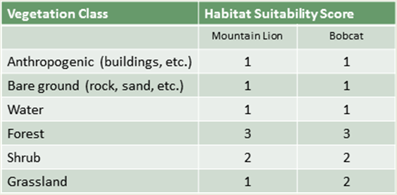
We used the reclassify tool (Spatial Analyst Tools/Reclass/Reclassify) to create two new vegetation maps, one ranking suitable habitat for bobcats and another for mountain lions.
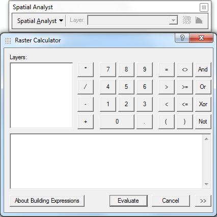
Raster Calculator:
Now that we have our two separate vegetation maps we need to create new vegetation rasters that are just in the area of the bobcat and mountain lion buffers. To do this we used raster calculator and the analysis mask. You can set your anaylsis mask under Options in the Spatial Analyst Toolbar.

We set our mask to the particular buffer we wanted to analyze and then we would use the raster calculator to calculate a new raster that would just be to the extent of the mask. we did this for each bobcat and mountain lion buffer in each of the four study sites for a total of 8 vegetation rasters. Once all these rasters were created we copied the raster attribute table and compared the percentage of high, medium and low qulaity bobcat and mountain lion habitat in these four areas.
Question 2 Analysis:
Our second research question was what are the differences in potential domestic/wild felid interaction as determined by suitable habitat and how do these risks compare with human perceptions?
Selection and Export:
To start analyzing this question we decided to look at individual domestic cat buffers around parcels and anaylze the buffer area for suitable bobcat and mountain lion habitat. To begin we took out 4 parcel shapefile from, each containing 50 parcels and we subsampled 5 parcels from each study site resulting in 4 files containing 5 parcels each.
Buffer:
We then buffered each of the 4 files by the average home range radius of a domestic cat (100 m), but this time we did not dissolve when we buffered.
Join:
Once again we wanted to remove the parcel from the buffer polygon so we joined the two files.
Select and Export:
Once the files were unioned we selected only the individual buffer
polygons and exported them as a shapefile We did this for every individual cat buffer, resulting in 20 separate files.
Raster Calculator:
As in the analysis of our first question we used raster calculator and the analysis mask to analyze the amount of suitable bobcat and mountain lion habitat in each individual buffer. Once all the 20 rasters were created we copied the attributes and compared the percentage of high, medium and low quality bobcat and mountain lion habitat in the buffers. We then averaged the 5 buffers in each area together to determine a mean percetage of habitat that we could compare across our four study sites.