GIS Analyses

Here are the basic questions we want to answer:

Since human impact varies across land ownership type, how does land ownership type (National Park, National Forest, and State Park) affect the density of jams? In posing this question, we are working from the assumptions: A) there are fewer upstream flow diversions in Rocky Mountain National Park than in Arapahoe-Roosevelt National Forest and B) there is less road access to streams in the National Park setting than in the National Forest or State Park.

How does recreational access affect jam density? To answer this question, we are using driving distance on roads as a proxy for recreational access. The driving distance analysis is outlined below in the cost-path analysis.

Cluster Analysis: Land Ownership Type's Effect on Jam Density

To see how land ownership jursidictional boundaries affect jam density, we used ArcGIS Spatial Analyst Neighborhood Statistics function to do a basic cluster analysis. We had three different categories of land ownership: State Park (Eldorado Canyon), National Forest (Arapahoe-Roosevelt), and National Park (Rocky Mountain). There were 19 field sites, which were created from polygons of a 150m stream buffer. Within those 19 field sites, we had 292 logjam point locations. In spatial analyst, when defining our analysis environment, we set the spatial extent to the Channel-Spanning Jams point location layer and we did not use an analysis mask. Once in the Neighborhood Statistics tool, we used a 7 x 7 cell rectangular sampling grid. Below, we've pasted in a copy of the interface with the rest of our parameters:

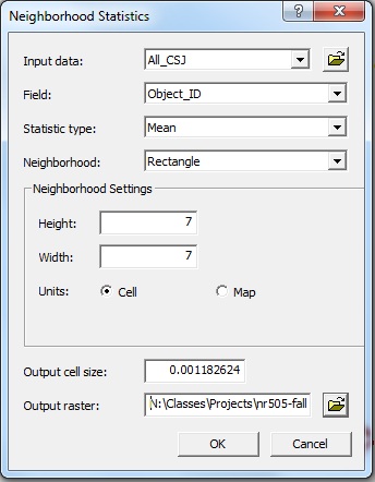
For more information on the Spatial Analyst Neighborhood Statistics function, see our "GIS Concepts" section.

Recreational Access: Cost-Path Distance and Road Density Analysis

To infer the level of recreational access to each of our field sites, we created road density raster layers to serve as our cost surface. A cost surface is required for Cost-distance modeling as it provides the features over which travel takes place. The roads layer, once rasterized, was the surface over which we wanted to model travel. Where there were roads, the value attribute table would contain a low impedence value for travel (a value of 1) and where there were no roads, the impedence to travel was high (100).

Roads along the Colorado Front Range as raster data.

We then used municipal boundaries and field cites as "region groups" for starting location and end destination, respectively. The output was a raster file with travel routes and associated path costs. Please see our "Results" section for the output of this cost-path analysis and for the output of the Cluster analysis introduced above.

Road density analysis was also conducted to obtain a visual depiction of the amount of road stretches along or near the field sites. The tool used was Spatial Analyst's "Density Analyst" function. The output raster file is included in the "Results" section and the steps for this process are outlined in the "Flowchart" section of our website.