The objective of this project is to determine the topographic and vegetation similarities and differences between the Hayman Fire (2002) and the High Park Fire (2012). These are two of the largest wildland forest fires in Colorado’s recent history, both occurring on the Front Range. Each fire burned in June, and continued to burn for close to a month. For the project, we analyzed the topography in each burn area; specifically, we chose to analyze the slope and aspect, as these are known to impact fire behavior. Further analysis was performed to determine patterns of slope and aspect within high severity burn areas. Additionally, we chose to analyze the vegetation in each burn area through the Normalized Difference Vegetation Index.
The Hayman Fire burned for twenty days in June of 2002. It burned areas in Douglas, Jefferson, Park and Teller counties in the central Front Range of Colorado. By the time the fire was extinguished, just over 117,000 acres was burned (Finney et al. 2003). The final fire perimeter included 138,114 acres (Finney et al. 2003). Of this area, 85% was National Forest land, 9 % was private land, 6 % was City of Denver land, and <1% was State land (Finney et al. 2003).
The High Park fire burned in Larimer County, Colorado in June 2012. According to the Incident Information System, the final fire perimeter included 87, 284 acres (2012). Of this area, 48.8% was Forest Service land, 45.3 % was private land, 5.8% was State owned land, and <0.1% was Bureau of Land Management or Bureau of Reclamation land (Incident Information System 2012).
Burn boundaries of High Park and Heyman, and Colorado Counties.
Note! Google Earth Plugin is not supported by Chrome 64-bit version. If you are using Chrome 64-bit version, please try a 32-bit version or other browsers, eg. Firefox, IE, and etc. to use the plugin. Or you can download the KML file and open it in Google Earth program to see the boundaries.
For this project, data was acquired from several sources. Burn boundaries were acquired from the high Park Fire Burned Area Emergency Response Team and U.S. Geological Survey. These files were used to clip other data and to define study area boundaries.
Digital Elevation Maps were also acquired from the U.S. Geological Survey. These files were published in 2013 and were all 1 ArcSecond IMG files. They were downloaded from The National Map Viewer, which can be accessed at viewer.nationalmap.gov/viewer
The final data downloaded for this project was imagery from LandSat. Also courtesy of the U.S. Geological Survey, LandSat data can be acquired using the USGS Global Visualization Viewer. This viewer can be accessed at glovis.usgs.gov
The burn severity map for the Hayman Fire was acquired from the United States Forest Service. Group members made contact with a Forest Service employee, who chose to share a fire severity shapefile with the group. Severity for this file was based upon percent tree mortality. The burn severity map for the High Park Fire was acquired from the Burned Areas Emergency Response Team. For the High Park Fire, severity was based upon a soil burn index. Since the two severity maps have different measures of severity, comparisons cannot be made directly, but can still give some ideas about relationships with other fire characteristics.
Many original files from data sources were in different projected coordinate systems or geographic coordinate systems. Some files were projected and exported to our database, while other were projected within map documents as needed. All analyses including area or measurements were done in UTM Zone 13N (NAD 1983).
Many files had to be created, in order to conduct our comparison between the two fires. The elevation source files were used to create raster files of slope, aspect and hillshade. The LandSat imagery was used to create Normalized Difference Vegetation Index files. The methodology for new file creation and analysis can be found on the Methodology Page of this website.
These created files were used for analyses with intersection, raster calculators, etc. Any other files created were as the results of those analyses
Data Sharing
In order to share data for this project, a Google Drive was often used. It seemed to be the simplest way to share data between group members. When on one’s personal computer, it is simple to connect the Google Drive to the computer. When you can do this, you can work “live’ on the drive and connect to the Drive folder on ArcCatalog and ArcGIS. Unfortunately, on Colorado State University’s network computers, one cannot connect to a persona or shared Google Drive folder. This meant that when utilizing C.S.U.’s computers, one would have to download files from the drive, conduct analyses or GIS functions, then upload files back to the Google Drive. This can be problematic as shapefiles contain multiple separate files, and raster files can have extra metadata text files associated with them as well. When moving data frequently, this multitude of files can make it easy for parts to be lost, and the files to lose function. Eventually, a group file was created on a shared network drive, which allowed all members to access data without transferring files. The structure can be seen here.
Data Naming Convention
In order to keep clarity with many different data files, one naming convention system was used. Every file began with a three letters that described which fire the file related to; for the Hayman fire, all files began with “hay” and for the High Park Fire, all files began with “HPF.” These letters were always followed by an underscore with a descriptive second part of name to describe what the file displayed. The Data Dictionary explains the names and descriptions of each file. As stated earlier, many original files from data sources were in different projected coordinate systems or geographic coordinate systems. Some files were projected and exported to our database, while other were projected within map documents as needed. All analyses including area or measurements were done in UTM Zone 13N (NAD 1983).
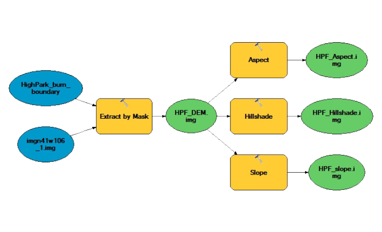
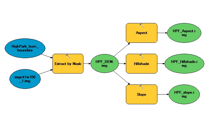
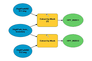
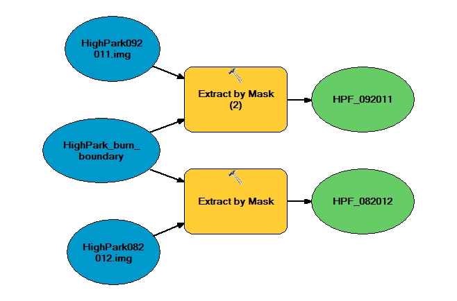
Using the downloaded elevation files from the U.S.G.S., the first step was to clip files to burn boundaries. This was done using the “extract by mask” tool. Next, we created three new rasters for each fire; these were the aspect, hillshade, and slope files. Each of these tools (aspect, hillshade and slope) create an output raster file. See figure 1 for the model displaying methods of extraction and raster creation for the High Park Fire. Remember, the High Park Fire original files were not projected, so the burn boundary has “UTM13” at the end of its name to confirm the projected file was used.
Slope and Aspect
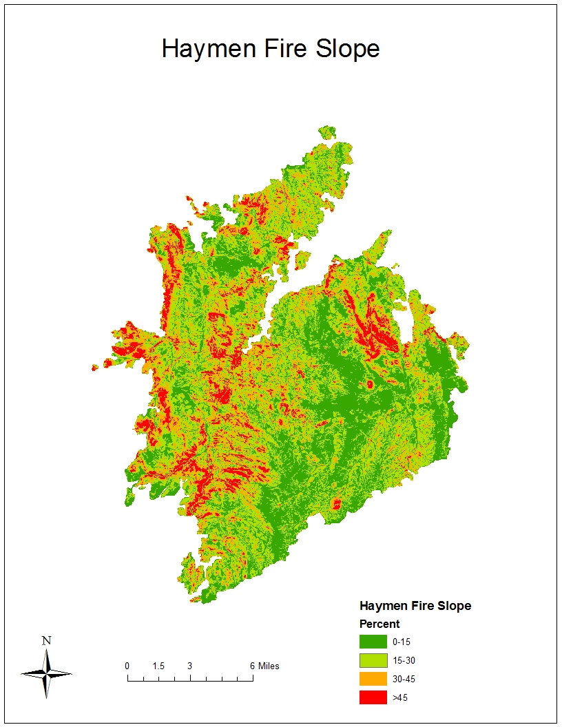
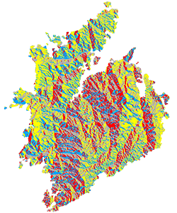
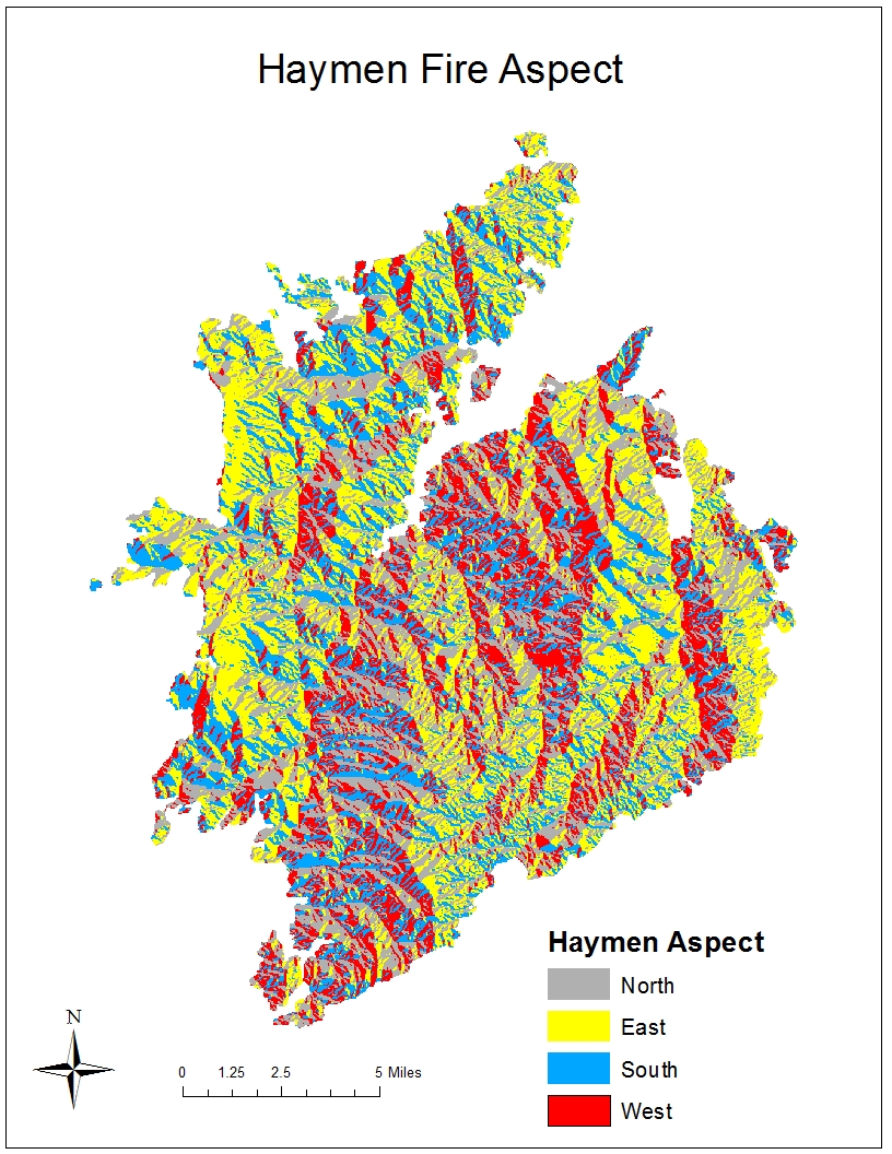
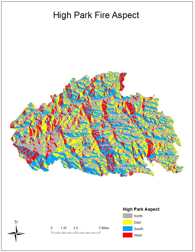
The slope and aspect raster files were then reclassified into four categories for each (0-15 degrees, 15-30 degrees, 30-45 degrees, and above 45 degrees for the slope; East, South, West, and North for the aspect) using the reclassify tool.
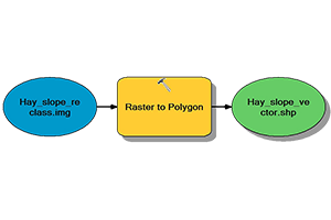
The reclassified rasters were then converted into a vector for further analysis.
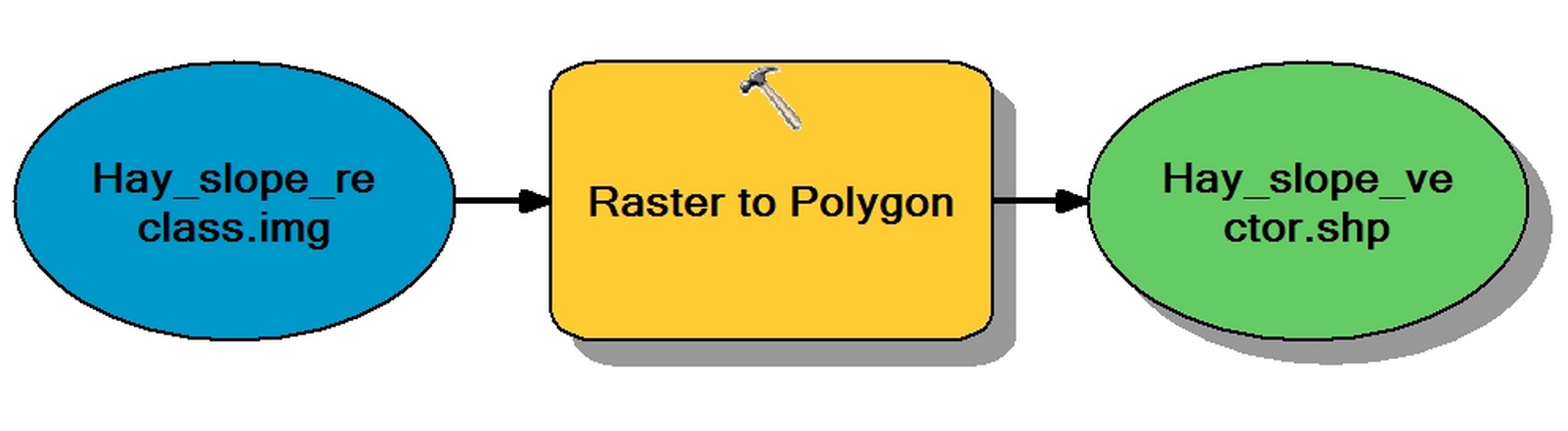
Using the Select by Attribute tool the individual slope and aspect shapefiles were generated for each category. These steps were repeated for both of the fires. We then created some graphical representation of slope and aspect for both fires. These was an even distribution of both slope and aspect when looking at the entire fires
Burn Severity
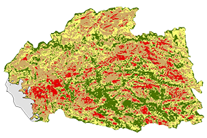
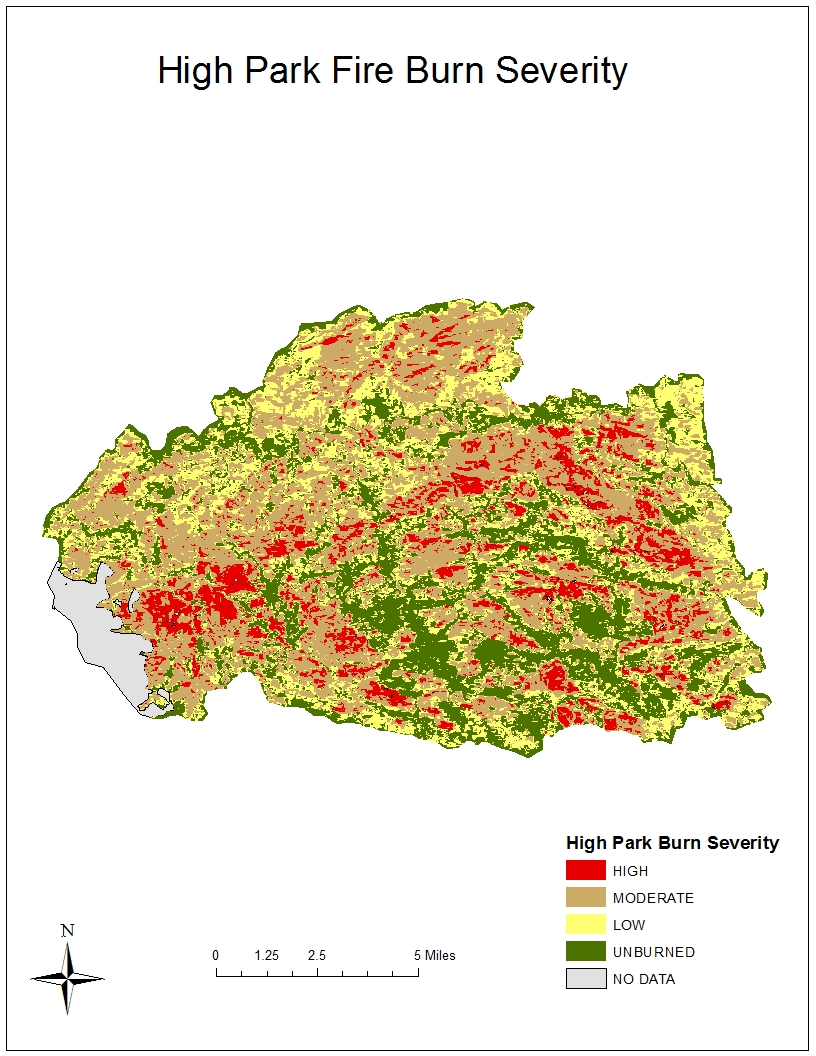
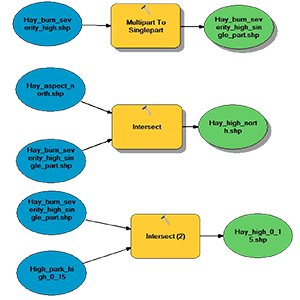
The next step was to determine if there were any patterns associated with high severity, slope, and aspect. In order to do this we needed to isolate the high severity portion of our burn severity layers. First, the burn severity layers needed to be dissolved. Next, the Select by Attribute tool was used to create a new layer of just high severity areas. This layer was then converted from multipart to singlepart using the the Multipart to Singlepart tool. Eventually, each aspect and slope classification was isolated within the high severity area.
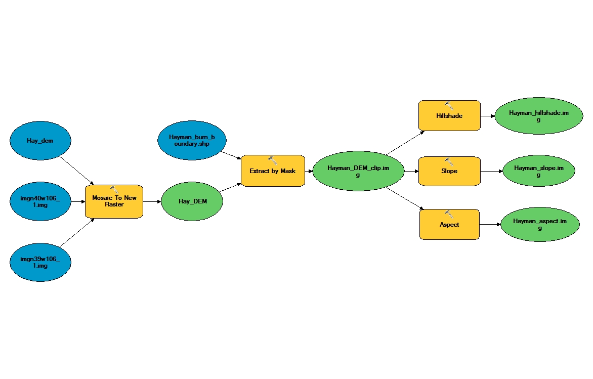
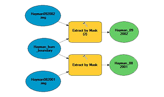
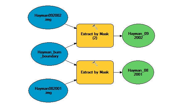
The vegetation analyses utilized Landsat imagery. Imagery was downloaded for two dates for each fire. One image was downloaded from the August before the fire, and the second image was from the September post-fire. We chose these files, because they were close enough in season, to eliminate any vegetation differences due to growing season. As both fires occurred in June, September was as soon after the fire as could be downloaded with high quality data. The first step, as with the topographic analyses, was to extract these files by the burn boundaries. See figure 3 for a model displaying extraction of the High Park Fire imagery, and see figure 4 for a model displaying extraction of the Hayman Fire imagery.
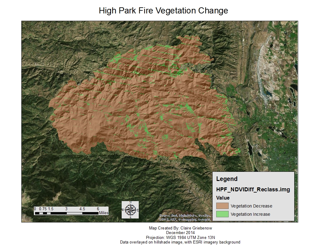
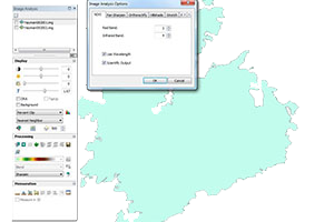
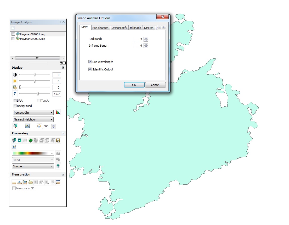
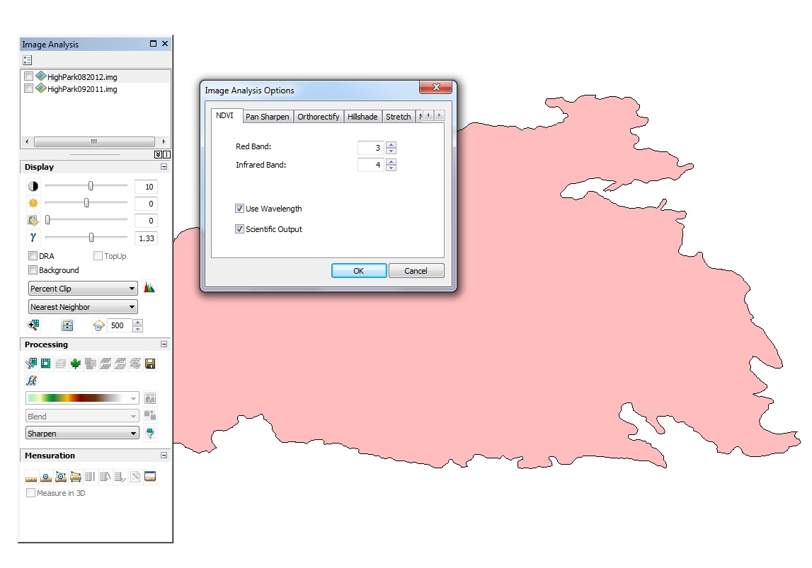
After clipping the LandSat imagery to fire boundaries, for each date, the Normalized Difference Vegetation Index was calculated. This can be done from the “Image Analysis” window of ArcGIS. From this window, one must first set the “Image Analysis Options” so that the Red Band is represented by band 3 and the Infared Band is represented by band 4. After setting these options, one can simply press the NDVI icon to create an NDVI layer for each image. This was done four times, once for each of the two dates for each of the two fires. Figure 5 shows this window and icon for the High Park Fire, and figure 6 shows this window and icon for the Hayman Fire.
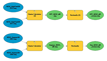
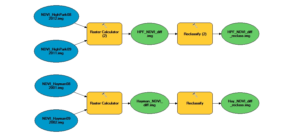
After creation of NDVI layer files, these files can be used to calculate the difference in vegetation before and after the fire. To do this, raster calculator and reclassify were used, see figure 7 for a model displaying the steps to create a vegetation difference for each fire. The raster calculator equation was the NDVI layer post-fire minus the NDVI layer pre-fire. Then, the result would give the difference in vegetation, showing a negative number where vegetation decreased and a positive number where vegetation increased. These files were then reclassified to a binary 1 or 0 showing an increase or decrease in vegetation.
LandSat imagery was used to analyze the vegetation change pre- and post-fires. In order to minimize seasonal bias, the image dates were from the August prior to each fire and the September following each fire (each fire occurred in June). As expected, there was significant amounts of vegetation loss with both fires (see Table below). The Hayman fire showed a decrease in over 99% of the area within the burned boundary. The High Park fire showed a decrease in over 91% of the area within the burned boundary. As the severity maps were created by different methods, it is difficult to infer a relationship between burn severity and vegetation increase or decrease, and compare directly between the two fires. Figures 8 and 9 display maps of the burned areas and their vegetation change.
| Fire Area | Decreased Veg (ac) | Percent | Increased Veg (ac) | Percent |
|---|---|---|---|---|
| Hayman | 128716.46 | 99.55% | 585.76 | 0.45% |
| High Park | 83302.04 | 91.86% | 7385.32 | 8.14% |
Aspect
30% of high severity areas were on east facing slopes. 21% of high severity areas were on west slopes. 24% of high severities were on south slopes. 25% of high severity areas were on north facing slopes. This information suggests that aspect was not a significant factor in determining fire severity for the Hayman fire.
Slope
38% of high severity areas were on slopes of 0-15%. 26% of high severities were on slopes of 15-30%. 27% of high severity areas were on slopes of 30-45%. 8% of high severity areas were on slopes of greater than 45%. This information suggests that slopes greater than 45% were less likely to burn at high severity. No other patterns can clearly be established with high severity areas and slope for the Hayman Fire.
Aspect
39% of high severity areas were on east facing slopes. 27% of high severity areas were on west slopes. 13% of high severities were on south slopes. 21% of high severity areas were on north facing slopes. This information suggests that easts facing slopes were most likely to burn at high severity and south facing slopes were less likely to burn at high severity. No other patterns were identified with aspect and fire severity for the High Park Fire.
Slope
39% of high severity areas were on east facing slopes. 27% of high severity areas were on west slopes. 13% of high severities were on south slopes. 21% of high severity areas were on north facing slopes. This information suggests that easts facing slopes were most likely to burn at high severity and south facing slopes were less likely to burn at high severity. No other patterns were identified with aspect and fire severity for the High Park Fire.
Weather, topography, and fuels are the three major characteristics which alter fire behavior. In this project, we analyzed the differences in topography of the Hayman and High Park Fires, and how slope or aspect affected fire severity. We did not find any major differences in the topography and severity relationships. In addition, we analyzed the percent vegetation cover loss between the two sites; these were not significantly different either. Without on-the-ground pre-fire fuels data, we cannot conduct a more extensive analysis of the fuels similarities or differences between these two fires.
With similar terrain characteristics and forest types, we are left to weather as a major characteristic which could have affected fire behavior. According to Reinhardt et al., “weather (fuel moisture and wind) is far more important than fuels in determining fire behavior [...] this is especially true if fires burning under moderate conditions are effectively suppressed, so that most acres burn under extreme conditions” (Reinhardt, 2008). Agee and Skinner choose the Hayman Fire as a case study for examining the effectiveness of fuel treatments (Agee and Skinner 2005). They determined that under less severe weather conditions, fuel treatments may have altered fire severity (Agee and Skinner 2005). These studies, as well as our GIS analyses, lead us to believe that any differences in severity or fire size were likely due to weather, suppression resources, and suppression challenges as opposed to topography in the case of the Hayman and High Park Fires.